A First Posterior with NLE

This tutorial trains a Neural Likelihood Estimator (NLE) on a linear-Gaussian simulator and samples the posterior with PyMC and NumPyro. The simulator is deliberately simple: its likelihood is a known Gaussian, so every step can be checked against an exact answer. The workflow is the same four phases used for any real simulator, Simulate → Train → Validate → Export, and the core pipeline is about twenty lines of setu code.

Running this notebook requires the pymc and numpyro extras (see the install how-to).

import arviz as az
import jax
import jax.numpy as jnp
import matplotlib.pyplot as plt
import numpy as np
import pandas as pd
import pymc as pm

import setu
from setu.integration.pymc import to_pymc

# Shared setu-docs figure style: applied when this notebook is executed by the
# docs build (setu_docs_style is on the build's PYTHONPATH); skipped harmlessly
# when the notebook is run standalone.
try:
    from setu_docs_style import set_style

    set_style()
except ImportError:
    pass

The simulator

The simulator draws an observation from a Gaussian centered on a shifted parameter vector,

\[x \mid \theta \sim \mathcal{N}(\theta + s, \Sigma),\]

with a standard normal prior \(\theta \sim \mathcal{N}(0, I)\) in three dimensions. setu ships this as setu.linear_gaussian(), one of its test simulators. Because prior and likelihood are conjugate, the exact posterior is a Gaussian with a closed-form mean and covariance, which makes this the ideal first problem: the entire neural pipeline can be compared against ground truth at the end.

One detail is worth flagging immediately: the parameter dimension and the observation dimension are both 3. That makes it impossible for setu to catch a swapped theta/x argument by shape, a point this tutorial returns to below.

theta_dim = x_dim = 3
shift = jnp.array([0.5, -0.5, 1.0])
likelihood_cov = 0.5 * jnp.eye(x_dim)
prior_mean = jnp.zeros(theta_dim)
prior_cov = jnp.eye(theta_dim)

key = jax.random.key(0)
k_simulate, k_create, k_fit, k_val, k_validate, k_obs = jax.random.split(key, 6)

Phase 1: Simulate

setu.simulate_dataset() builds a training set from two functions: a prior_fn that draws a single parameter vector from a key, and a simulator_fn that maps one (theta, key) pair to one observation. Both are jax.vmap-ed internally over n_samples fresh keys.

The library helpers have slightly different signatures, so two thin wrappers adapt them: setu.sample_prior() draws a whole batch (here a batch of one), and setu.linear_gaussian() takes its key as the last of four arguments. Passing everything by keyword keeps the adaptation explicit.

def prior(key):
    return setu.sample_prior(mean=prior_mean, cov=prior_cov, n_samples=1, key=key)[0]


def simulator(theta, key):
    return setu.linear_gaussian(theta=theta, shift=shift, cov=likelihood_cov, key=key)


dataset = setu.simulate_dataset(simulator, prior, n_samples=50_000, key=k_simulate)
dataset.theta.shape, dataset.x.shape

((50000, 3), (50000, 3))

The observed data

Inference needs something to infer from. A known ground-truth parameter \(\theta^*\) generates ten observed Trials; the goal of the rest of the tutorial is to recover \(\theta^*\) from these ten observations alone, and the known value makes the recovery checkable.

theta_true = jnp.array([0.8, -0.3, 0.2])
obs_keys = jax.random.split(k_obs, 10)
x_obs = jax.vmap(lambda k: simulator(theta_true, k))(obs_keys)
x_obs.shape

(10, 3)

Phase 2: Train

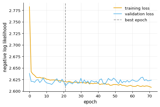
setu separates model construction from training: setu.create_nle() builds an untrained estimator (by default a neural spline flow), and setu.fit_nle() trains it with early stopping on a held-out validation split. The returned setu.TrainingResult carries the trained estimator together with the loss history.

nle = setu.create_nle(x_dim=x_dim, theta_dim=theta_dim, key=k_create)
result = setu.fit_nle(nle, dataset, max_epochs=400, show_progress=False, key=k_fit)
nle = result.nle

print(
    f"stopped at epoch {len(result.losses)}, best epoch {result.best_epoch}, "
    f"best validation loss {result.val_losses[result.best_epoch]:.3f}"
)

stopped at epoch 72, best epoch 21, best validation loss 2.611

fig, ax = plt.subplots()
ax.plot(result.losses, label="training loss")
ax.plot(result.val_losses, label="validation loss")
ax.axvline(result.best_epoch, color="#999999", linestyle="--", label="best epoch")
ax.set(xlabel="epoch", ylabel="negative log likelihood")
ax.legend()
plt.show()

A note on argument order

The trained estimator evaluates \(\log p(x \mid \theta)\) via nle.log_prob(x, theta), with the observation first. The sampling and export functions take theta first. In this problem x_dim == theta_dim, so swapping the two arguments raises no error and returns a finite, plausible, wrong number:

lp_correct = nle.log_prob(x=x_obs[0], theta=theta_true)
lp_swapped = nle.log_prob(x=theta_true, theta=x_obs[0])

print(f"log p(x | theta)   = {lp_correct:.3f}")
print(f"swapped arguments  = {lp_swapped:.3f}   (finite, plausible, wrong)")

log p(x | theta)   = -1.864
swapped arguments  = -10.119   (finite, plausible, wrong)

Whenever the parameter and observation dimensions match, only the argument order distinguishes the two, and a silent swap corrupts every downstream result. Passing x= and theta= by keyword, as done throughout this tutorial, removes the failure mode entirely.

Phase 3: Validate

A learned likelihood is not trusted until it is checked. Validation runs on a fresh dataset that played no role in training. The result.validate() convenience runs the standard battery: training diagnostics, C2ST (a classifier tries to tell estimator samples from simulator samples; accuracy near 0.5 means indistinguishable), MMD, sliced-Wasserstein, likelihood SBC (a rank-calibration check on the learned density), and a likelihood-accuracy check.

val = setu.simulate_dataset(simulator, prior, n_samples=1_000, key=k_val)
val_data = setu.ValidationDataset(theta=val.theta, x=val.x)

validation = result.validate(val_data, key=k_validate)
print(validation.summary())

Estimator Validation: PASSED
----------------------------------------
Training: WARN
  Marginal training: loss reduced 6.3% (epoch 22/72). Consider more training.
C2ST (marginal): PASS
  C2ST=0.511 (n=1000): distributions indistinguishable
MMD: PASS
  MMD=0.0000 (n=1000): distributions similar
Sliced-Wasserstein: PASS
  SW=0.0956 (n=1000): distributions similar
Likelihood SBC: PASS
  SBC KS D=0.0220 (ranks uniform, well-calibrated)
Likelihood Accuracy: PASS
  Likelihood preference rate 0.903 (estimator correctly prefers true theta)

Warnings:
  - Training: Marginal training: loss reduced 6.3% (epoch 22/72). Consider more training.

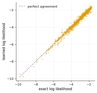
Because this simulator has a tractable likelihood, a more direct check is also available here (and only here): evaluating the learned and the exact log-density on the same validation pairs. On a real problem this plot does not exist, which is exactly why the checks above matter.

exact_lp = jax.vmap(
    lambda x, theta: setu.analytical_log_likelihood(
        x=x, theta=theta, shift=shift, cov=likelihood_cov
    )
)(val.x, val.theta)
learned_lp = jax.vmap(nle.log_prob)(val.x, val.theta)

fig, ax = plt.subplots(figsize=(4.5, 4.5))
ax.scatter(exact_lp, learned_lp, s=8, alpha=0.4)
lims = [float(exact_lp.min()), float(exact_lp.max())]
ax.plot(lims, lims, color="#999999", linestyle="--", label="perfect agreement")
ax.set(xlabel="exact log likelihood", ylabel="learned log likelihood")
ax.legend()
plt.show()

Phase 4: Export to PyMC

Export produces a likelihood term inside an ordinary PyMC model: to_pymc wraps the trained estimator as a potential attached to any PyMC random variable. Priors, transformations, and sampling all remain plain PyMC. With nuts_sampler="blackjax" the whole model graph is compiled to JAX; the default NUTS sampler works as well but calls back into Python on every step. chain_method="vectorized" runs the chains as one vectorized computation, which is what a single device (one CPU or GPU) needs, and random_seed makes the run reproducible.

with pm.Model():
    theta = pm.Normal("theta", mu=0.0, sigma=1.0, shape=theta_dim)
    to_pymc(nle, theta=theta, x_observed=x_obs)
    idata = pm.sample(
        draws=500,
        tune=500,
        chains=4,
        nuts_sampler="blackjax",
        nuts_sampler_kwargs={"chain_method": "vectorized"},
        progressbar=False,
        random_seed=0,
    )

az.summary(idata, var_names=["theta"])

	mean	sd	hdi_3%	hdi_97%	mcse_mean	mcse_sd	ess_bulk	ess_tail	r_hat
theta[0]	0.765	0.206	0.368	1.139	0.005	0.005	2065.0	1144.0	1.0
theta[1]	-0.023	0.221	-0.454	0.379	0.005	0.005	1947.0	1267.0	1.0
theta[2]	-0.115	0.219	-0.519	0.281	0.005	0.005	1844.0	1678.0	1.0

Checking against the exact posterior

With a Gaussian prior and a Gaussian likelihood, the posterior after \(n\) observations is Gaussian with precision and mean

\[\Lambda = \Sigma_0^{-1} + n\,\Sigma^{-1}, \qquad \mu_{\text{post}} = \Lambda^{-1}\Big(\Sigma_0^{-1}\mu_0 + \Sigma^{-1}\textstyle\sum_i (x_i - s)\Big).\]

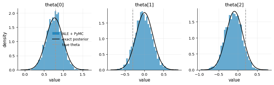
Overlaying it on the sampled posterior closes the loop: the samples came from a neural approximation of the likelihood, yet they should trace the exact answer.

n_obs = x_obs.shape[0]
post_prec = jnp.linalg.inv(prior_cov) + n_obs * jnp.linalg.inv(likelihood_cov)
post_cov = jnp.linalg.inv(post_prec)
post_mean = post_cov @ (
    jnp.linalg.inv(prior_cov) @ prior_mean
    + jnp.linalg.inv(likelihood_cov) @ (x_obs - shift).sum(axis=0)
)

pymc_samples = idata.posterior["theta"].values.reshape(-1, theta_dim)

fig, axes = plt.subplots(1, 3, figsize=(10, 3.2))
for d, ax in enumerate(axes):
    ax.hist(
        pymc_samples[:, d],
        bins=40,
        density=True,
        alpha=0.6,
        color="#0072B2",
        label="NLE + PyMC",
    )
    sd = float(jnp.sqrt(post_cov[d, d]))
    grid = np.linspace(post_mean[d] - 4 * sd, post_mean[d] + 4 * sd, 200)
    pdf = np.exp(-0.5 * ((grid - float(post_mean[d])) / sd) ** 2)
    pdf /= sd * np.sqrt(2 * np.pi)
    ax.plot(grid, pdf, color="#000000", label="exact posterior")
    ax.axvline(
        float(theta_true[d]), color="#999999", linestyle="--", label="true theta"
    )
    ax.set(title=f"theta[{d}]", xlabel="value")
axes[0].set(ylabel="density")
axes[0].legend(fontsize=9)
fig.tight_layout()
plt.show()

Export to NumPyro

The same trained estimator exports to NumPyro without retraining; this is what Amortized means in practice. NumPyro is JAX-native, so to_numpyro adds the log-likelihood directly as a factor with no bridge layer. Reproducibility works differently from PyMC: the random state is an explicit rng_key passed to mcmc.run.

import numpyro
import numpyro.distributions as dist
from numpyro.infer import MCMC, NUTS

from setu.integration.numpyro import to_numpyro


def model():
    theta = numpyro.sample("theta", dist.Normal(jnp.zeros(theta_dim), 1.0).to_event(1))
    to_numpyro(nle, theta=theta, x_observed=x_obs)


mcmc = MCMC(
    NUTS(model),
    num_warmup=500,
    num_samples=500,
    num_chains=4,
    chain_method="sequential",
    progress_bar=False,
)
mcmc.run(jax.random.key(1))
numpyro_samples = np.asarray(mcmc.get_samples()["theta"])

Both PPL paths agree with the closed-form posterior mean up to a small residual that reflects the approximation error of the learned likelihood (more training simulations shrink it). All three sit near the ground-truth parameter, differing from it by the posterior’s own uncertainty, since ten observations only pin \(\theta\) down so far:

pd.DataFrame(
    {
        "exact posterior mean": np.asarray(post_mean),
        "PyMC mean": pymc_samples.mean(axis=0),
        "NumPyro mean": numpyro_samples.mean(axis=0),
        "true theta": np.asarray(theta_true),
    },
    index=[f"theta[{d}]" for d in range(theta_dim)],
).round(3)

	exact posterior mean	PyMC mean	NumPyro mean	true theta
theta[0]	0.771	0.765	0.775	0.8
theta[1]	0.003	-0.023	-0.027	-0.3
theta[2]	-0.090	-0.115	-0.120	0.2

Where to go next

The four phases above transfer unchanged to simulators whose likelihood is genuinely intractable; only the validation scatter plot against the exact density goes away. Tutorial 2 applies the workflow to real experimental data with a discrete outcome (MixedNLE). What is SBI? gives the conceptual background for the four phases, and the API reference documents every function used here.