Reed Frogs: A Discrete Likelihood Validated Against an Exact Binomial

This notebook reproduces the multilevel tadpole survival analysis from McElreath’s Statistical Rethinking (Ch. 13), using real experimental data from Vonesh & Bolker (2005). The setup: 48 tanks of reed frog tadpoles (Hyperolius spinigularis) with varying initial densities, predator treatments, and tadpole sizes. The outcome is the number of survivors.

The survivor count is a pure discrete observation, so the estimator here is DiscreteNLE – a neural likelihood for discrete data (a CategoricalMADE over the count, conditioned on the initial density). Because the Binomial likelihood is tractable, we can fit the exact model in PyMC and compare it against the learned one. If DiscreteNLE has learned the likelihood well, both approaches recover matching posteriors. This validates the neural likelihood bridge before moving to intractable simulators in the next notebook.

Outline:

1. Load and explore the data

2. Exact PyMC model: hierarchical Binomial with varying intercepts

3. Add predator effect and observe variance reduction

4. Train a DiscreteNLE on simulated count data and validate it

5. Replace pm.Binomial with the DiscreteNLE and compare posteriors

import arviz as az
import jax
import jax.numpy as jnp
import matplotlib.pyplot as plt
import numpy as np
import pandas as pd
import pymc as pm

import setu

# Shared setu-docs figure style: applied when this notebook is executed as a
# docs tutorial (setu_docs_style is on the build's PYTHONPATH); skipped
# harmlessly when the notebook is run standalone from examples/.
try:
    from setu_docs_style import set_style

    set_style()
except ImportError:
    pass

The data

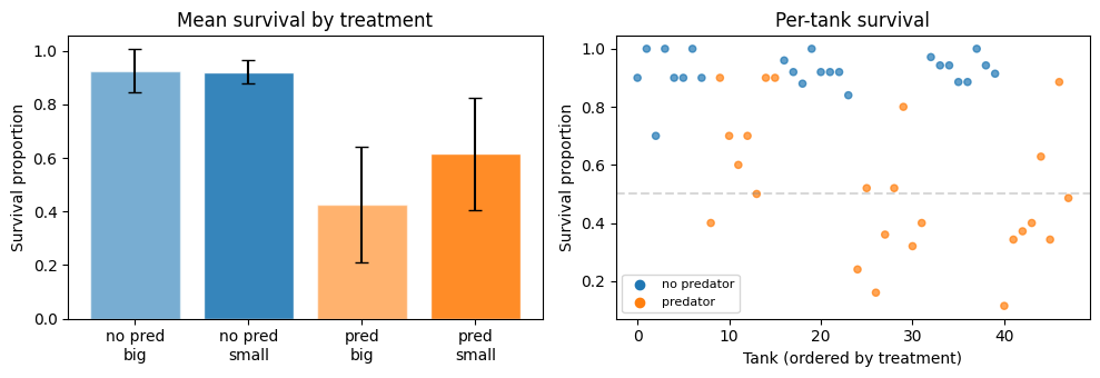
The dataset comes from Vonesh & Bolker (2005), studying predation on African reed frog tadpoles. The experiment used a 3 x 2 x 2 factorial design:

Factor	Levels
Initial density	10, 25, 35 tadpoles per tank
Predator	present / absent
Tadpole size	big / small

Each of the 12 treatment combinations has 4 replicate tanks, giving 48 tanks total. Each tank records the number of survivors.

frogs = pd.read_csv("data/reedfrogs.csv")
n_tanks = len(frogs)
density = frogs["density"].values
survivors = frogs["surv"].values
predator = (frogs["pred"] == "pred").astype(int).values
size = (frogs["size"] == "small").astype(int).values
frogs.head(10)

	density	pred	size	surv	propsurv
0	10	no	big	9	0.9
1	10	no	big	10	1.0
2	10	no	big	7	0.7
3	10	no	big	10	1.0
4	10	no	small	9	0.9
5	10	no	small	9	0.9
6	10	no	small	10	1.0
7	10	no	small	9	0.9
8	10	pred	big	4	0.4
9	10	pred	big	9	0.9

fig, axes = plt.subplots(1, 2, figsize=(10, 3.5))

# Left: survival proportion by treatment
ax = axes[0]
for i, (pred_val, pred_label) in enumerate([(0, "no predator"), (1, "predator")]):
    for j, (sz_val, sz_label) in enumerate([(0, "big"), (1, "small")]):
        mask = (predator == pred_val) & (size == sz_val)
        props = survivors[mask] / density[mask]
        x_pos = i * 2 + j
        ax.bar(
            x_pos,
            props.mean(),
            yerr=props.std(),
            capsize=4,
            color=f"C{i}",
            alpha=0.6 + 0.3 * j,
            edgecolor="w",
        )
ax.set_xticks(range(4))
ax.set_xticklabels(["no pred\nbig", "no pred\nsmall", "pred\nbig", "pred\nsmall"])
ax.set(ylabel="Survival proportion", title="Mean survival by treatment")

# Right: raw survival by tank, ordered by treatment
ax = axes[1]
colors = ["C0" if p == 0 else "C1" for p in predator]
ax.scatter(range(n_tanks), survivors / density, c=colors, s=20, alpha=0.7)
ax.axhline(0.5, color="gray", ls="--", alpha=0.3)
ax.set(
    xlabel="Tank (ordered by treatment)",
    ylabel="Survival proportion",
    title="Per-tank survival",
)
# Manual legend
ax.scatter([], [], c="C0", label="no predator")
ax.scatter([], [], c="C1", label="predator")
ax.legend(fontsize=8)

fig.tight_layout()

Model 1: varying intercepts

Following McElreath (Ch. 13), the first model uses a hierarchical Binomial with partial pooling over tanks. Each tank \(j\) has its own survival log-odds \(\alpha_j\), drawn from a shared population distribution:

\[ S_j \sim \mathrm{Binomial}(N_j,\, p_j), \qquad \mathrm{logit}(p_j) = \alpha_j \]

\[ \alpha_j \sim \mathrm{Normal}(\bar\alpha,\, \sigma), \qquad \bar\alpha \sim \mathrm{Normal}(0,\, 1.5), \qquad \sigma \sim \mathrm{Exponential}(1) \]

A non-centered parameterization (\(\alpha_j = \bar\alpha + \sigma z_j\), \(z_j \sim \mathrm{Normal}(0,1)\)) helps the sampler.

with pm.Model() as model_intercepts:
    a_bar = pm.Normal("a_bar", 0, 1.5)
    sigma = pm.Exponential("sigma", 1)
    z = pm.Normal("z", 0, 1, shape=n_tanks)
    alpha = pm.Deterministic("alpha", a_bar + z * sigma)
    p = pm.math.sigmoid(alpha)
    pm.Binomial("obs", n=density, p=p, observed=survivors)

    trace_intercepts = pm.sample(
        draws=2000,
        tune=1000,
        chains=4,
        nuts_sampler="blackjax",
        nuts_sampler_kwargs={"chain_method": "vectorized"},
        progressbar=False,
        random_seed=0,
    )

az.summary(trace_intercepts, var_names=["a_bar", "sigma"])

	mean	sd	hdi_3%	hdi_97%	mcse_mean	mcse_sd	ess_bulk	ess_tail	r_hat
a_bar	1.345	0.256	0.890	1.854	0.007	0.004	1416.0	2727.0	1.0
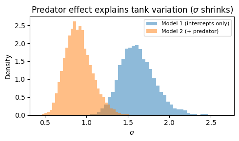
sigma	1.618	0.212	1.228	2.017	0.005	0.003	1816.0	3439.0	1.0

Model 2: add predator effect

Predators dramatically reduce survival. Adding a predator coefficient \(\beta_P\) should explain part of the between-tank variation, causing \(\sigma\) to shrink:

\[ \mathrm{logit}(p_j) = \alpha_j + \beta_P \cdot P_j, \qquad \beta_P \sim \mathrm{Normal}(0,\, 0.5) \]

with pm.Model() as model_predator:
    a_bar = pm.Normal("a_bar", 0, 1.5)
    sigma = pm.Exponential("sigma", 1)
    beta_pred = pm.Normal("beta_pred", 0, 0.5)
    z = pm.Normal("z", 0, 1, shape=n_tanks)
    alpha = pm.Deterministic("alpha", a_bar + z * sigma + beta_pred * predator)
    p = pm.math.sigmoid(alpha)
    pm.Binomial("obs", n=density, p=p, observed=survivors)

    trace_predator = pm.sample(
        draws=2000,
        tune=1000,
        chains=4,
        nuts_sampler="blackjax",
        nuts_sampler_kwargs={"chain_method": "vectorized"},
        progressbar=False,
        random_seed=0,
    )

az.summary(trace_predator, var_names=["a_bar", "sigma", "beta_pred"])

	mean	sd	hdi_3%	hdi_97%	mcse_mean	mcse_sd	ess_bulk	ess_tail	r_hat
a_bar	2.195	0.224	1.794	2.635	0.004	0.003	2944.0	4634.0	1.0
sigma	0.909	0.164	0.614	1.222	0.003	0.002	2446.0	3917.0	1.0
beta_pred	-1.826	0.303	-2.377	-1.250	0.006	0.004	2328.0	3950.0	1.0

fig, ax = plt.subplots(figsize=(5, 3))
ax.hist(
    trace_intercepts.posterior["sigma"].values.flatten(),
    bins=40,
    density=True,
    alpha=0.5,
    label="Model 1 (intercepts only)",
)
ax.hist(
    trace_predator.posterior["sigma"].values.flatten(),
    bins=40,
    density=True,
    alpha=0.5,
    label="Model 2 (+ predator)",
)
ax.set(
    xlabel=r"$\sigma$",
    ylabel="Density",
    title=r"Predator effect explains tank variation ($\sigma$ shrinks)",
)
ax.legend(fontsize=8)
fig.tight_layout()

setu DiscreteNLE: learning the likelihood from simulations

Now we replace the exact pm.Binomial with a learned likelihood. The survivor count \(S\) is discrete, so we use DiscreteNLE – there is no continuous channel to model. The approach:

1. Simulate training data. A Binomial simulator outputs the survivor count \(S\); the initial density \(N\) enters as a condition.

2. Train the DiscreteNLE. A CategoricalMADE models \(p(S \mid \alpha, N)\) over the possible counts \(0, \dots, 35\).

3. Validate. Before trusting the likelihood, validate() checks calibration (SBC), sample quality (C2ST, total variation), and likelihood accuracy on held-out simulations.

4. Plug into PyMC. The trained estimator replaces the Binomial likelihood.

If the DiscreteNLE learns the Binomial well, the posteriors should match the exact model. This is the validation step before trusting a learned likelihood on problems where no exact likelihood exists.

Step 1: simulate training data

def binomial_simulator(theta, key, conditions):
    """Simulate the survivor count from a Binomial model."""
    n = conditions[0].astype(jnp.int32)
    p = jax.nn.sigmoid(theta[0])
    count = jax.random.binomial(key, n=n, p=p)
    # Pure-discrete observation: the survivor count. The initial density N
    # enters as a condition, not as part of the observation.
    return jnp.array([count], dtype=jnp.float32)


def prior_fn(key):
    """Broad prior over logit survival, wider than the hierarchical prior."""
    return jax.random.normal(key, (1,)) * 3.0


def conditions_fn(key):
    """Draw a random initial density from {10, 25, 35}."""
    options = jnp.array([10.0, 25.0, 35.0])
    idx = jax.random.randint(key, (), 0, 3)
    return jnp.array([options[idx]])


key = jax.random.key(42)
n_sims = 50_000
key, k_data = jax.random.split(key)
dataset = setu.simulate_dataset(
    binomial_simulator, prior_fn, n_sims, k_data, conditions_fn=conditions_fn
)
dataset.theta.shape, dataset.x.shape, dataset.conditions.shape

<string>:6: UserWarning: x appears to be integer-valued. Consider DiscreteNLE for pure discrete data or MixedNLE for mixed continuous/discrete data instead of NLE.

((50000, 1), (50000, 1), (50000, 1))

Step 2: train the DiscreteNLE

key, k_dnle = jax.random.split(key)
discrete_nle = setu.create_discrete_nle(
    x_dim=1,
    theta_dim=1,
    distribution="categorical",
    num_categories=jnp.array([36]),  # survivor counts run 0..35
    condition_dim=1,  # initial density N
    key=k_dnle,
)

key, k_train = jax.random.split(key)
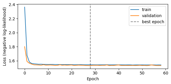
result = setu.fit_discrete_nle(
    discrete_nle, dataset, key=k_train, max_epochs=300, max_patience=30
)

fig, ax = plt.subplots(figsize=(6, 3))
ax.plot(result.losses, label="train")
ax.plot(result.val_losses, label="validation")
ax.axvline(result.best_epoch, color="k", ls="--", alpha=0.5, label="best epoch")
ax.set(xlabel="Epoch", ylabel="Loss (negative log-likelihood)")
ax.legend()
fig.tight_layout()

Step 3: validate before trusting the likelihood

A learned likelihood must be checked before it replaces the exact one. validate() draws a fresh set of simulations and runs calibration and sample-quality diagnostics: likelihood-SBC (rank calibration), C2ST and total variation (do estimator samples match the simulator?), and likelihood accuracy (does the estimator prefer the true parameters?). MMD and Sliced-Wasserstein are skipped – they assume continuous data.

from setu.validation import ValidationDataset

key, k_val, k_check = jax.random.split(key, 3)
val_raw = setu.simulate_dataset(
    binomial_simulator, prior_fn, 5_000, k_val, conditions_fn=conditions_fn
)
val_data = ValidationDataset(
    theta=val_raw.theta, x=val_raw.x, conditions=val_raw.conditions
)

report = result.validate(val_data, k_check)
print(report.summary())

Estimator Validation: PASSED
----------------------------------------
Training: PASS
  Loss reduced 34.8% (epoch 29/59)
C2ST (marginal): PASS
  C2ST=0.511 (n=1000): distributions indistinguishable
Likelihood SBC: PASS
  SBC KS D=0.0106 (ranks uniform, well-calibrated)
Total Variation: PASS
  TV=0.0790 (n=1000): PMFs similar
Likelihood Accuracy: PASS
  Likelihood preference rate 0.898 (estimator correctly prefers true theta)

Step 4: hierarchical inference with the DiscreteNLE likelihood

The trained DiscreteNLE is plugged into the same hierarchical structure. pm.Binomial is replaced by to_pymc_hierarchical, which evaluates the learned log-likelihood for each tank given its parameters and density condition. We fit Model 2 (with predator effect) for comparison.

trained_dnle = result.discrete_nle

# One survivor count per tank -> (n_tanks, x_dim=1); setu auto-expands the
# missing trial axis. Shapes are subject-first: axis 0 indexes tanks.
x_observed = survivors.astype(np.float32)[:, None]
cond_observed = density.astype(np.float32)[:, None]

with pm.Model() as dnle_model:
    a_bar = pm.Normal("a_bar", 0, 1.5)
    sigma = pm.Exponential("sigma", 1)
    beta_pred = pm.Normal("beta_pred", 0, 0.5)
    z = pm.Normal("z", 0, 1, shape=n_tanks)
    alpha = pm.Deterministic("alpha", a_bar + z * sigma + beta_pred * predator)

    # alpha is (n_tanks,); DiscreteNLE expects (n_tanks, theta_dim=1)
    trained_dnle.to_pymc_hierarchical(
        alpha[:, None],
        x_observed,
        conditions=cond_observed,
        subject_dim="tank",
    )

    # nuts_sampler="blackjax" keeps the whole step in JAX (no PyTensor
    # per-step overhead); chain_method="vectorized" runs all chains in one
    # vmapped program on a single device; progressbar=False is required with
    # vectorized BlackJAX (its IO callback breaks under vmap).
    trace_dnle = pm.sample(
        draws=2000,
        tune=1000,
        chains=4,
        nuts_sampler="blackjax",
        nuts_sampler_kwargs={"chain_method": "vectorized"},
        progressbar=False,
        random_seed=0,
    )

az.summary(trace_dnle, var_names=["a_bar", "sigma", "beta_pred"])

	mean	sd	hdi_3%	hdi_97%	mcse_mean	mcse_sd	ess_bulk	ess_tail	r_hat
a_bar	2.189	0.224	1.772	2.608	0.005	0.003	2465.0	3617.0	1.0
sigma	0.898	0.169	0.586	1.212	0.004	0.002	2253.0	3567.0	1.0
beta_pred	-1.833	0.301	-2.386	-1.266	0.007	0.004	2065.0	3003.0	1.0

Posterior comparison

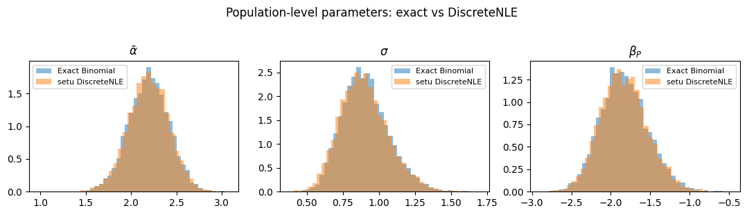
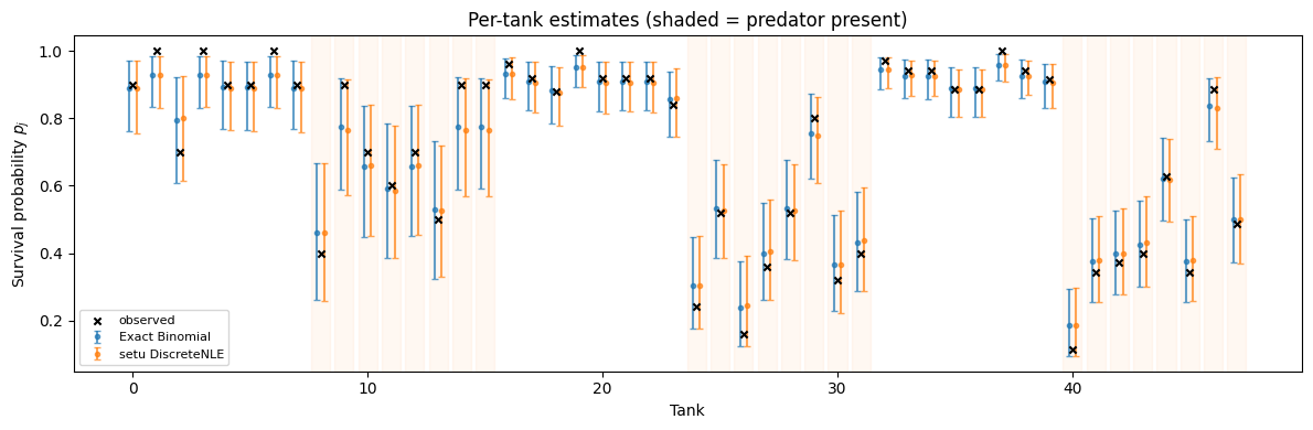
If the DiscreteNLE has learned the Binomial likelihood accurately, the posteriors from both approaches should overlap.

fig, axes = plt.subplots(1, 3, figsize=(11, 3))
params = {"a_bar": r"$\bar\alpha$", "sigma": r"$\sigma$", "beta_pred": r"$\beta_P$"}
for i, (var, label) in enumerate(params.items()):
    exact = trace_predator.posterior[var].values.flatten()
    dnle_post = trace_dnle.posterior[var].values.flatten()
    axes[i].hist(exact, bins=40, density=True, alpha=0.5, label="Exact Binomial")
    axes[i].hist(dnle_post, bins=40, density=True, alpha=0.5, label="setu DiscreteNLE")
    axes[i].set(title=label)
    axes[i].legend(fontsize=8)
fig.suptitle("Population-level parameters: exact vs DiscreteNLE", y=1.02)
fig.tight_layout()

# Per-tank survival probabilities: posterior mean +/- 90% CI
alpha_exact = trace_predator.posterior["alpha"].values.reshape(-1, n_tanks)
alpha_dnle = trace_dnle.posterior["alpha"].values.reshape(-1, n_tanks)
p_exact = 1 / (1 + np.exp(-alpha_exact))
p_dnle = 1 / (1 + np.exp(-alpha_dnle))

fig, ax = plt.subplots(figsize=(12, 4))
tanks = np.arange(n_tanks)
for samples, label, offset in [
    (p_exact, "Exact Binomial", -0.15),
    (p_dnle, "setu DiscreteNLE", 0.15),
]:
    mean = samples.mean(axis=0)
    lo, hi = np.percentile(samples, [5, 95], axis=0)
    ax.errorbar(
        tanks + offset,
        mean,
        yerr=[mean - lo, hi - mean],
        fmt="o",
        ms=3,
        capsize=2,
        label=label,
        alpha=0.7,
    )

# Observed proportions
ax.scatter(
    tanks, survivors / density, marker="x", color="k", s=20, label="observed", zorder=5
)

# Shade by predator treatment
for j in range(n_tanks):
    if predator[j]:
        ax.axvspan(j - 0.4, j + 0.4, color="C1", alpha=0.05)

ax.set(
    xlabel="Tank",
    ylabel="Survival probability $p_j$",
    title="Per-tank estimates (shaded = predator present)",
)
ax.legend(fontsize=8, loc="lower left")
fig.tight_layout()

Summary

The DiscreteNLE posteriors closely match the exact Binomial posteriors for the population-level hyperparameters (\(\bar\alpha\), \(\sigma\), \(\beta_P\)) and the 48 tank-level survival probabilities. Key observations:

• Partial pooling: Both models show shrinkage of extreme tanks toward the population mean, especially in the low-density group.

• Predator effect: \(\beta_P\) is strongly negative (~\(-2\)), and including it reduces the residual tank variance \(\sigma\).

• Validated before use: SBC, C2ST, total variation, and likelihood accuracy all pass on held-out simulations, so the learned likelihood is trustworthy before it enters the sampler.

• Discrete data, no continuous channel: modeling the survivor count directly with DiscreteNLE matches the exact discrete likelihood.

This validates setu’s neural likelihood bridge on a problem with known ground truth. The next notebook replaces the tractable Binomial with a mechanistic individual-based simulator where the likelihood is intractable. The same setu workflow applies; only the simulator changes.