How fast is setu, and on what

setu is JAX-native: a learned likelihood and its gradient compile into one fused kernel with no per-call dispatch overhead. This page measures what that buys, and where it stops mattering. Every number comes from one benchmark task and is scoped to it.

Note

These benchmarks are run on a single 3D linear-Gaussian model with three free parameters and a Gaussian likelihood with known shift and covariance. The task is deliberately left simple so the exact posterior is available in closed form and a fast posterior can be checked for correctness. Throughout, the NLE we used here is a masked autoregressive flow (three transforms, width-64 hidden layers). CPU results are from an Apple M3 Pro, GPU results from a Tesla V100. A different task, model size, or device would move these curves; this is not a general performance claim.

The comparison is against sbi, the reference PyTorch package for simulation-based inference: two setu paths (setu + NumPyro, setu + PyMC/BlackJAX) against two sbi paths (sbi + Pyro, sbi + PyMC), with the exact likelihood as the reference floor.

Show code cell source

Hide code cell source

import numpy as np
import pandas as pd
import matplotlib.pyplot as plt

from matplotlib.ticker import FuncFormatter, LogLocator, NullFormatter
from matplotlib_inline.backend_inline import set_matplotlib_formats

from setu_docs_style import set_style

set_style()
set_matplotlib_formats("svg")  # crisp vector figures at any zoom

# Plain, trailing-zero-free tick labels: 10 not 10^1, 0.5 not 0.50.
_plain = FuncFormatter(lambda v, _pos: f"{v:g}")


def log_ticks(ax, minor_y: bool = False) -> None:
    """Label log axes with plain numbers; optionally add 2/5 intermediate ticks."""
    ax.xaxis.set_major_formatter(_plain)
    ax.xaxis.set_minor_formatter(NullFormatter())
    if ax.get_yscale() == "log":
        ax.yaxis.set_major_formatter(_plain)
        if minor_y:
            ax.yaxis.set_minor_locator(LogLocator(base=10.0, subs=(2.0, 5.0)))
            ax.yaxis.set_minor_formatter(_plain)
            ax.tick_params(axis="y", which="minor", labelsize=8)
        else:
            ax.yaxis.set_minor_formatter(NullFormatter())


# Committed benchmark runs: per-eval and MCMC on CPU, per-eval on GPU.
pereval = pd.read_csv("../../benchmarks/results/2026-03-10_114708.csv")
mcmc = pd.read_csv("../../benchmarks/results/mcmc_2026-03-12_222240.csv")
cuda = pd.read_csv("../../benchmarks/results/cuda_2026-03-10_130546.csv")

# This page presents the flat (single-level) 3D linear-Gaussian task only.
pereval = pereval[pereval["level"] == "flat"]
mcmc = mcmc[mcmc["level"] == "flat"]

# Shared, colorblind-safe styling: setu paths in blues, sbi paths in warm
# tones, the exact reference in black. Legend order is fixed.
STYLE = {
    "true-likelihood": ("#000000", "x", "true likelihood", (2, 1)),
    "setu-numpyro": ("#0072B2", "o", "setu + NumPyro", None),
    "setu-pymc": ("#56B4E9", "s", "setu + PyMC/BlackJAX", None),
    "sbi-pyro": ("#E69F00", "^", "sbi + Pyro", None),
    "sbi-pymc": ("#D55E00", "v", "sbi + PyMC", None),
}
ORDER = list(STYLE)

Per-evaluation: one log-likelihood and its gradient

A single MCMC step needs one log-likelihood and its gradient. This times that call (100 repetitions) as the number of observations grows; both axes are logarithmic, and lower is faster.

Show code cell source

Hide code cell source

grad = pereval[pereval["with_grad"] == True]  # noqa: E712 (pandas mask)

fig, ax = plt.subplots(figsize=(6.4, 4.2))
for runner in ORDER:
    sub = grad[grad["runner"] == runner].sort_values("n_trials")
    if sub.empty:
        continue
    color, marker, label, dashes = STYLE[runner]
    line, = ax.plot(sub["n_trials"], sub["median_ms"], color=color, marker=marker,
                    markersize=5, linewidth=1.5, label=label)
    if dashes:
        line.set_dashes(dashes)

ax.set(xscale="log", yscale="log", xlabel="observations conditioned on",
       ylabel="log-likelihood + gradient (ms)")
log_ticks(ax, minor_y=True)
ax.legend(loc="upper left", fontsize=9)
fig.tight_layout()

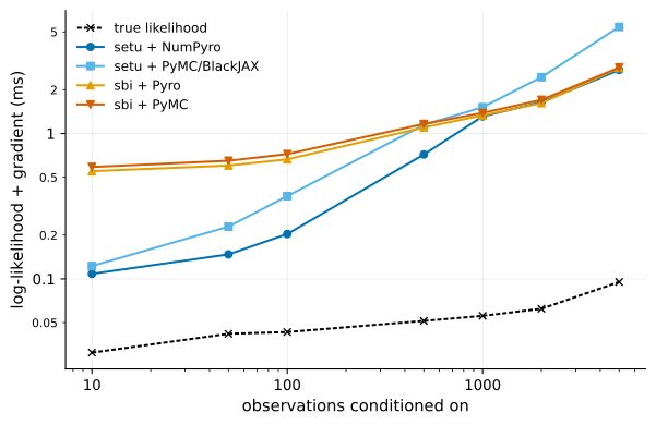
At 10 observations setu costs about 0.1 ms against sbi’s 0.55 ms. The gap closes as the count grows: by 1000 observations setu + NumPyro and sbi + Pyro nearly coincide, and setu + PyMC/BlackJAX is slower than sbi at the largest sizes. The end-to-end runs show the same shape.

End-to-end: a full MCMC run

What a user actually waits for is a full posterior. This times a complete run (500 tuning steps, 500 draws, two chains), taking the median wall-clock over ten repetitions.

Show code cell source

Hide code cell source

wall = (mcmc.groupby(["runner", "n_trials"])["wall_clock_s"]
        .median().reset_index())

fig, ax = plt.subplots(figsize=(6.4, 4.2))
for runner in ORDER:
    sub = wall[wall["runner"] == runner].sort_values("n_trials")
    if sub.empty:
        continue
    color, marker, label, dashes = STYLE[runner]
    line, = ax.plot(sub["n_trials"], sub["wall_clock_s"], color=color, marker=marker,
                    markersize=5, linewidth=1.5, label=label)
    if dashes:
        line.set_dashes(dashes)

ax.set(xscale="log", yscale="log", xlabel="observations conditioned on",
       ylabel="wall-clock time (s)")
log_ticks(ax, minor_y=True)
ax.legend(loc="upper left", fontsize=9)
fig.tight_layout()

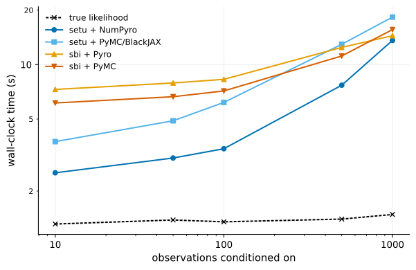
The picture matches the per-call one: at 10 observations setu + NumPyro takes 2.5 s against sbi + PyMC at 6.1 s (2.4x), narrowing to 13.6 s against 15.6 s (1.15x) at 1000. The advantage is real at the small-to-medium scales most hierarchical models occupy and shrinks toward parity as the problem grows. setu + PyMC/BlackJAX turns slower than both sbi paths beyond a few hundred observations, so setu + NumPyro is the path to cite.

Fast is only useful if it is also correct

Speed is worthless if the posterior is wrong. Because this task has a closed-form posterior, each run is scored with C2ST: a classifier trained to separate sampled draws from exact posterior draws, where 0.5 means indistinguishable and higher means the sampler has drifted.

Show code cell source

Hide code cell source

quality = mcmc[mcmc["c2st"].notna()]
c2st = (quality.groupby(["runner", "n_trials"])["c2st"]
        .median().reset_index())

fig, ax = plt.subplots(figsize=(6.4, 4.2))
ax.axhspan(0.45, 0.55, color="#999999", alpha=0.18, label="indistinguishable")
ax.axhline(0.5, color="#999999", linewidth=0.8, linestyle="--")
for runner in ORDER:
    sub = c2st[c2st["runner"] == runner].sort_values("n_trials")
    if sub.empty:
        continue
    color, marker, label, dashes = STYLE[runner]
    line, = ax.plot(sub["n_trials"], sub["c2st"], color=color, marker=marker,
                    markersize=5, linewidth=1.5, label=label)
    if dashes:
        line.set_dashes(dashes)

ax.set(xscale="log", xlabel="observations conditioned on", ylabel="C2ST (0.5 is ideal)",
       ylim=(0.45, 1.0))
log_ticks(ax)
ax.legend(loc="upper left", fontsize=9)
fig.tight_layout()

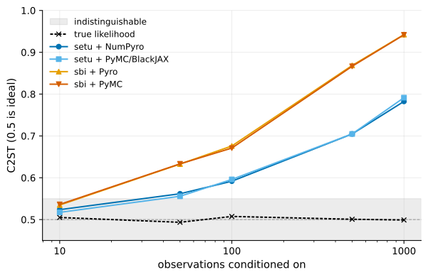
At small counts every sampler is indistinguishable from exact (near 0.5). The score rises with observations for all of them: as more data sharpens the posterior, the estimator’s finite fidelity shows against an ever-tighter target. This is a property of the learned likelihood, not the sampler. setu stays at least as close to exact as sbi throughout, and closer at the large end (about 0.78 against 0.94 at 1000). The speed comparison is therefore between posteriors of equal or better quality, not a speed-for-accuracy trade.

Why the gap narrows on CPU but holds on the GPU

One mechanism explains every curve above. A log-likelihood call is fixed overhead plus arithmetic. At small observation counts overhead dominates: Python dispatch, framework bookkeeping, and the boundary crossing into the numerical backend on every step. JAX pays that overhead once by compiling the whole call into a single fused kernel, so setu wins widest exactly where overhead is the entire cost. At large counts the flow’s forward and backward arithmetic dominates instead, and that arithmetic is identical in both frameworks, so the fixed-overhead saving shrinks as a share of the total and the CPU curves converge.

On a GPU the same mechanism widens the gap rather than closing it. The plot tracks how many times faster setu + NumPyro is than sbi + Pyro per call, on each device.

Show code cell source

Hide code cell source

def speedup(df, fast, slow):
    f = df[df["runner"] == fast].set_index("n_trials")["median_ms"]
    s = df[df["runner"] == slow].set_index("n_trials")["median_ms"]
    common = sorted(set(f.index) & set(s.index))
    return common, [s[n] / f[n] for n in common]

gpu = cuda[(cuda["level"] == "flat") & (cuda["with_grad"] == True)]  # noqa: E712
cpu_x, cpu_y = speedup(grad, "setu-numpyro", "sbi-pyro")
gpu_x, gpu_y = speedup(gpu, "setu-numpyro", "sbi-pyro-cuda")

fig, ax = plt.subplots(figsize=(6.4, 4.2))
ax.plot(gpu_x, gpu_y, color="#0072B2", marker="s", markersize=5, linewidth=1.5,
        label="GPU (Tesla V100)")
ax.plot(cpu_x, cpu_y, color="#D55E00", marker="o", markersize=5, linewidth=1.5,
        label="CPU (Apple M3 Pro)")
ax.axhline(1.0, color="#999999", linewidth=0.8, linestyle="--")
ax.set(xscale="log", ylim=(0, None), xlabel="observations conditioned on",
       ylabel="setu speedup (sbi time / setu time)")
log_ticks(ax)
ax.legend(loc="center right", fontsize=9)
fig.tight_layout()

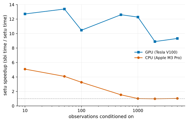
On CPU the speedup falls from about 5x to parity as observations grow. On the GPU it stays near 10x and does not narrow, because sbi’s PyTorch path launches thirty to fifty separate kernels per step and pays launch latency on each, while setu compiles the whole computation into one XLA program. The catch is that this model is far too small to need a GPU: a 30k-parameter flow on 3D data is trivial arithmetic, so both frameworks are actually slower on the GPU than on the CPU in absolute terms, and the workload never grows large enough to make the GPU the bottleneck. The GPU result is therefore an argument about architecture, not a reason to reach for one here. The GPU runs also sweep parallel versus sequential chains and hierarchical scales, produced by the code in the repository’s benchmarks/.

Why there is no sbi-plus-BlackJAX comparison

A fair like-for-like would also run sbi through BlackJAX, JAX’s NUTS sampler. It cannot be done: sbi wraps its estimator in PyTensor operators backed by PyTorch, and BlackJAX requires every operator in the graph to be JAX-traceable, which a PyTorch-backed operator is not. This is structural, not a missing feature. setu is JAX-native, so exporting a learned likelihood into a fully JAX-compiled sampler is the default path, and the benchmark compares setu’s JAX paths against the JAX paths sbi can actually reach.

Scope and caveats

• One task. A 3D linear-Gaussian model. A higher parameter dimension, a larger flow, or a genuinely intractable simulator would each move the curves; they do not generalize on their own.

• setu + NumPyro is the fast path. setu + PyMC/BlackJAX is convenient for staying inside PyMC but is not the one to cite for speed at scale.

• The learned likelihood has finite fidelity. The C2ST rise is a real limit of neural likelihood estimation, and the reason setu treats validation as a required step, not an afterthought.

The benchmark code and configurations that produced these numbers are in the repository’s benchmarks/.

Where to go next

Why validate a learned likelihood covers the calibration checks between a trained estimator and a trusted posterior. Why hierarchical inference is powerful shows where the small-to-medium scales setu favors arise. The shape conventions reference covers the hierarchical layouts the full benchmark also measures.