
Why hierarchical inference is powerful#
Scientific data usually arrives in groups. The Reed Frog experiment of Vonesh and Bolker (2005), the running example in Tutorial 2, stocked 48 tanks with tadpoles and recorded how many survived in each. Every tank is its own small survival experiment, and the scientific question is per tank: what is the survival probability in this tank? The 48 tanks are not unrelated, though. They are tadpoles of the same species under variations of one protocol, so what is learned in one tank should inform the others. How to encode that “should” is the subject of this page, and the answer is the reason setu carries a hierarchical shape convention at all.
Note
The pooled/unpooled/hierarchical arc used here is adapted from a 2025 EuroSciPy
talk, janfb/pyro-meets-sbi,
re-grounded on the tadpole tanks so the whole site shares one running example.
A point estimate hides what a posterior shows#
Take one tank of 10 tadpoles with 9 survivors. The maximum-likelihood estimate of its survival probability is the observed fraction, 0.9. Reported alone, that number claims a precision it does not have: 10 animals cannot pin a probability to a single value. Bayesian inference reports the full range instead. Given a prior \(p(\theta)\) and the Binomial likelihood \(p(x \mid \theta)\), it returns the posterior
a distribution over survival probabilities rather than one point. A PPL such as PyMC or NumPyro draws that posterior with MCMC once the model is written as priors plus a likelihood. The question is what the model says about 48 tanks at once.
Three ways to model 48 tanks#
Complete pooling assumes one survival probability shared by every tank. It estimates a single number from all 48 tanks together, which makes it precise but blind: real tanks differ by density, predator treatment, and tadpole size, and a single rate cannot represent that spread. For the Reed Frog data the pooled rate is about 0.70, a figure no individual tank is obliged to match.
No pooling goes to the opposite extreme: a separate, independent survival probability per tank, each estimated from that tank’s data alone. Nothing learned in one tank reaches any other. A tank of 10 animals is estimated as noisily as its 10 data points allow, and a tank where all 10 survived is estimated at exactly 1.0, a boundary value that reflects small-sample luck more than biology.
Partial pooling, the hierarchical model, sits between the two. Each tank keeps its own survival log-odds \(\alpha_j\), but those per-tank values are themselves drawn from a shared population distribution whose mean and spread are estimated jointly with the tanks:
The population distribution \(\mathrm{Normal}(\bar\alpha, \sigma)\) acts as a prior that the data itself informs. A tank with little data leans on it heavily; a tank with plenty of data barely notices it. That single mechanism is where the power comes from.
The power: borrowing strength#
Fitting the three models to the real tanks makes the difference concrete. The no-pooling estimate of each tank is its observed survival fraction; the hierarchical estimate is the posterior mean under partial pooling.
import numpy as np
import pandas as pd

from setu_docs_style import COLORS, set_style

palette = set_style()

frogs = pd.read_csv("../../examples/data/reedfrogs.csv")
density = frogs["density"].to_numpy()
survivors = frogs["surv"].to_numpy()
n_tanks = len(frogs)

# No pooling: each tank estimated from its own data alone.
p_nopool = survivors / density

# Complete pooling: a single rate shared by every tank.
p_pool = survivors.sum() / density.sum()

print(f"{n_tanks} tanks at densities {sorted(set(density.tolist()))}")
print(f"complete-pooling survival probability: {p_pool:.2f}")
print(f"no-pooling estimates range from {p_nopool.min():.2f} to {p_nopool.max():.2f}")
48 tanks at densities [10, 25, 35]
complete-pooling survival probability: 0.70
no-pooling estimates range from 0.11 to 1.00
import pymc as pm

with pm.Model():
    a_bar = pm.Normal("a_bar", 0.0, 1.5)
    sigma = pm.Exponential("sigma", 1.0)
    z = pm.Normal("z", 0.0, 1.0, shape=n_tanks)
    alpha = pm.Deterministic("alpha", a_bar + z * sigma)
    pm.Binomial("obs", n=density, p=pm.math.sigmoid(alpha), observed=survivors)

    trace = pm.sample(
        draws=1000,
        tune=1000,
        chains=4,
        nuts_sampler="blackjax",
        nuts_sampler_kwargs={"chain_method": "vectorized"},
        progressbar=False,
        random_seed=0,
    )

alpha_post = trace.posterior["alpha"].to_numpy().reshape(-1, n_tanks)
p_hier = (1.0 / (1.0 + np.exp(-alpha_post))).mean(axis=0)
p_bar = float((1.0 / (1.0 + np.exp(-trace.posterior["a_bar"].to_numpy()))).mean())
print(f"population-mean survival probability: {p_bar:.2f}")
population-mean survival probability: 0.79
Plotting the no-pooling and hierarchical estimates side by side, tank by tank, shows what partial pooling does to each one.
import matplotlib.pyplot as plt

tanks = np.arange(n_tanks)
fig, ax = plt.subplots(figsize=(9, 3.6))

# Faint segment from each no-pooling estimate to its hierarchical estimate.
ax.vlines(tanks, p_nopool, p_hier, color=COLORS["reference"], linewidth=0.8)
ax.scatter(tanks, p_nopool, s=26, color=COLORS["estimate"], label="no pooling")
ax.scatter(tanks, p_hier, s=26, color=COLORS["posterior"], label="hierarchical")
ax.axhline(p_bar, color=COLORS["true"], linestyle="--", linewidth=0.8,
           label="population mean")

# Density-group dividers: tanks are ordered 16 per density (10, 25, 35).
for boundary in (15.5, 31.5):
    ax.axvline(boundary, color=COLORS["reference"], linewidth=0.6, alpha=0.5)
for center, label in ((7.5, "density 10"), (23.5, "density 25"), (39.5, "density 35")):
    ax.text(center, 0.02, label, ha="center", fontsize=9, color=COLORS["reference"])

ax.set(xlabel="tank", ylabel="survival probability", ylim=(0.0, 1.05))
ax.legend(loc="lower right", ncol=2)
fig.tight_layout()
plt.show()
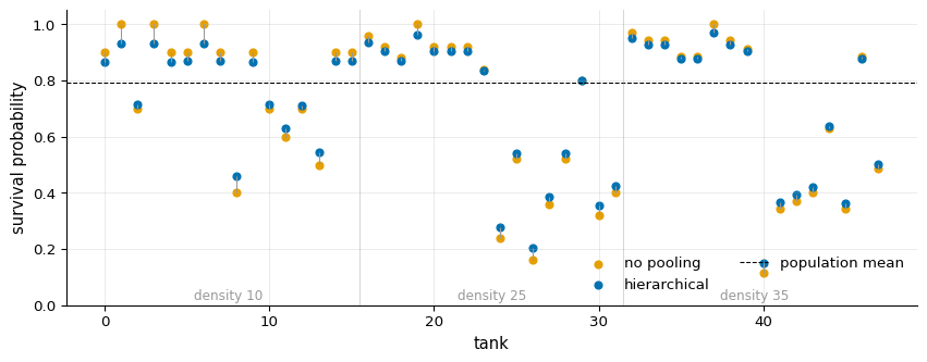
Every blue point has been pulled from its orange point toward the dashed population mean. This is shrinkage, and its size is not uniform: the smallest tanks, on the left at density 10, move the most, while the largest tanks on the right barely shift. A tank of 10 animals carries little information, so the population distribution dominates its estimate and drags it inward; a tank of 35 animals speaks mostly for itself. The tanks where all animals survived, estimated at exactly 1.0 with no pooling, are pulled back off that boundary toward the population mean.
toward_mean = np.abs(p_nopool - p_bar) - np.abs(p_hier - p_bar)
most_shrunk = np.argsort(toward_mean)[::-1][:5]
pd.DataFrame(
    {
        "tank": most_shrunk,
        "density": density[most_shrunk],
        "no pooling": p_nopool[most_shrunk].round(2),
        "hierarchical": p_hier[most_shrunk].round(2),
        "moved toward mean": toward_mean[most_shrunk].round(2),
    }
).set_index("tank")
| density | no pooling | hierarchical | moved toward mean | |
|---|---|---|---|---|
| tank | ||||
| 1 | 10 | 1.00 | 0.93 | 0.07 |
| 3 | 10 | 1.00 | 0.93 | 0.07 |
| 6 | 10 | 1.00 | 0.93 | 0.07 |
| 8 | 10 | 0.40 | 0.46 | 0.06 |
| 26 | 25 | 0.16 | 0.21 | 0.05 |
Shrinkage is not a distortion to be corrected; it is the model spending each tank’s evidence in proportion to how much of it there is. The consequences are practical. Extreme estimates from small samples are tempered toward what the rest of the data supports, so the fit generalizes better. Every tank contributes to the population distribution, which in turn sharpens every other tank, so the tanks borrow strength from one another. And because the population distribution is itself estimated, the model can predict a new tank that has not been observed at all, which neither pooling extreme can do.
Why the (G, S, T, *E) shape convention exists#
The hierarchy in that model has levels: individual trials nest inside tanks, and
tanks could themselves nest inside larger groups. setu encodes those levels
directly in array shapes, the (G, S, T, *E) convention, with groups and
Subjects / Groups outermost, Trials next, and the event
dimensions of a single observation last. The Reed Frog tanks are subjects, one
observation per tank, so the survivor data is subject-first and the same
estimator that handles this two-level case handles a flat single-level analysis
or a three-level one without reshaping. The hierarchical export helpers
vmap over those leading axes internally rather than looping in Python. The
shape conventions reference lays out the layouts for each
level.
When the likelihood is intractable#
Everything above rested on one convenience: the Binomial likelihood \(p(S_j \mid N_j, p_j)\) is known in closed form, so PyMC can evaluate it directly. That is exactly why Tutorial 2 can check setu against an exact answer. Real mechanistic models rarely offer the convenience. Replace the Binomial with an individual-based simulator of predation and metamorphosis, one that tracks animals through time, and the closed form disappears: the simulator still generates survivor counts, but it cannot report the probability of any particular count.
The hierarchical structure does not change, and it is no less desirable. What is
missing is only the likelihood term. This is where setu enters. Train a
likelihood Estimator on simulations, validate it,
and export it into the identical hierarchical model, where the
learned term stands in for pm.Binomial:
trained_discrete_nle.to_pymc_hierarchical(
    alpha[:, None], x_observed, conditions=cond_observed, subject_dim="tank"
)
The priors, the population distribution, the shrinkage, and the per-tank posteriors all remain. Only the one term that a simulator cannot supply is replaced by a learned one. That is the bridge setu builds, and hierarchical modeling is the reason it is worth building.
Where to go next#
Tutorial 2 runs this hierarchical model on the tadpole tanks end to end, comparing a learned DiscreteNLE likelihood against the exact Binomial. What is SBI? explains the Simulate → Train → Validate → Export workflow the bridge follows, and the glossary pins down the terms used here.