
Why validate a learned likelihood#
Training reports a loss, and the loss goes down. That is a statement about the optimizer, not about the estimator: a network can minimize its training objective and still assign miscalibrated probabilities to data it was never scored against. Because a learned likelihood is exported into a PPL and drives every posterior drawn from it, a miscalibration there propagates silently into the science. Validation is the phase that catches it, and it runs before any MCMC.
Validation is a loop, not a verdict#
validate_estimator runs a battery of diagnostics and reports each as pass,
warn, or fail. The output is a signal about a workflow step, never a judgment on
a method. The response to a check that lights up is mechanical:
Read which check fired and by how much.
Retrain with more simulations, or adjust the architecture, or widen the simulation proposal.
Re-run the same check.
A first fit that fails a check is an ordinary intermediate state, not a dead end. The remainder of this page makes one of those checks precise and then walks the loop once on a real fit.
What likelihood-level SBC checks#
SBC (simulation-based calibration) is the calibration check most specific to a density. setu’s SBC is likelihood-level: it interrogates the learned density \(p_{\text{est}}(x \mid \theta)\) directly, with no posterior and no MCMC. For each prior draw \(\theta_i\) paired with its true observation \(x^{\text{true}}_i\):
Sample \(n\) synthetic observations \(x_1, \dots, x_n \sim p_{\text{est}}(\cdot \mid \theta_i)\) from the learned likelihood.
Score every synthetic observation and the true observation under the estimator’s own
log_prob. For multi-trial data the per-trial log-probabilities are averaged over trials for \(x^{\text{true}}_i\) only; each synthetic \(x_j\) is a single draw scored once.Form the rank \(r_i = \#\{\, j : \log p_{\text{est}}(x_j) < \log p_{\text{est}}(x^{\text{true}}_i) \,\}\). On discrete observables (a DiscreteNLE over counts) many synthetic draws tie with the true value at the same
log_prob, so setu breaks ties with a random offset, \(r_i = \#\{<\} + \text{Uniform}\{0, \dots, \#\{=\}\}\) (inert for continuous data); without it a calibrated discrete estimator is under-ranked and fails SBC spuriously.After collecting one rank per \(\theta_i\), test those ranks for uniformity with a Kolmogorov-Smirnov test.
For single-trial data, a calibrated estimator makes the true observation exchangeable with its own synthetic draws, so its rank is uniform on \(\{0, \dots, n\}\) and the KS test sees a flat histogram. A miscalibrated density pushes the true data systematically high or low in the ranking, and the histogram develops a slope or a peak. One caveat follows from step 2: averaging over trials on \(x^{\text{true}}_i\) only narrows the true score relative to the single-draw synthetic scores, so with several trials the calibrated reference is no longer exactly uniform. On multi-trial data the rank test is therefore read comparatively, as movement between fits, rather than against a strict uniform.
The verdict uses the KS statistic \(D\) (the largest gap between the empirical
and uniform rank CDFs), not its p-value: with many \(\theta_i\) the p-value
rejects on negligible deviations, whereas \(D\) measures the size of the
miscalibration. The default thresholds warn at \(D = 0.05\) and fail at \(D = 0.10\);
only a fail flips the overall passed flag, and only strict=True turns a fail
into a raised ValidationError. The number of synthetic datasets per parameter
defaults to n_samples = 1000; the KS thresholds are the configurable part.
How this differs from posterior SBC#
Classical SBC, as introduced by Talts et al., is a posterior check: it draws \(\theta_i\) from the prior, simulates data, runs full inference to obtain a posterior for each simulated dataset, and ranks \(\theta_i\) within its posterior samples. That requires one MCMC run per simulated dataset, which is expensive precisely for a likelihood estimator, whose whole point is to be sampled inside a PPL. Amortized posterior methods (NPE) sidestep the cost because the posterior itself is amortized, so ranking is cheap. setu learns a likelihood, so its cheap analogue ranks the true data within the learned likelihood rather than a parameter within a posterior. Both detect miscalibration; they interrogate different objects. (NRE, which learns a ratio rather than a density, carries an analogous ratio-level rank check.)
SBC is also complementary to C2ST, the two-sample test that asks whether a classifier can tell estimator samples from simulator samples. An estimator can have accurate marginals, and so a near-chance C2ST, while still ranking true data non-uniformly under its own density. The example below is exactly that case.
For a DiscreteNLE, setu adds one more marginal check: the total variation distance between the estimator’s probability mass function and the simulator’s empirical PMF over the count values. It is the discrete counterpart of the sample-distance checks (MMD, Sliced-Wasserstein) that only apply to continuous data, and it warns at \(\text{TV} = 0.15\) and fails at \(0.25\).
Walking the loop once#
The linear-Gaussian simulator from Tutorial 1 makes the loop concrete because its cost is negligible. A first fit is deliberately starved of data: 100 simulations.
import jax
import jax.numpy as jnp

import setu
from setu_docs_style import COLORS, set_style

palette = set_style()

theta_dim = x_dim = 3
shift = jnp.array([0.5, -0.5, 1.0])
likelihood_cov = 0.5 * jnp.eye(x_dim)
prior_mean = jnp.zeros(theta_dim)
prior_cov = jnp.eye(theta_dim)


def prior(key):
    return setu.sample_prior(mean=prior_mean, cov=prior_cov, n_samples=1, key=key)[0]


def simulator(theta, key):
    return setu.linear_gaussian(theta=theta, shift=shift, cov=likelihood_cov, key=key)


key = jax.random.key(0)
k_train, k_create, k_fit, k_val, k_validate = jax.random.split(key, 5)

val = setu.simulate_dataset(simulator, prior, n_samples=1_000, key=k_val)
val_data = setu.ValidationDataset(theta=val.theta, x=val.x)

undertrained = setu.simulate_dataset(simulator, prior, n_samples=100, key=k_train)
nle = setu.create_nle(x_dim=x_dim, theta_dim=theta_dim, key=k_create)
result = setu.fit_nle(nle, undertrained, max_epochs=60, show_progress=False, key=k_fit)

validation_undertrained = result.validate(val_data, key=k_validate)
print(validation_undertrained.summary())
Estimator Validation: FAILED
----------------------------------------
Training: PASS
  Loss reduced 70.1% (epoch 37/60)
C2ST (marginal): PASS
  C2ST=0.550 (n=1000): distributions indistinguishable
MMD: PASS
  MMD=0.0325 (n=1000): distributions similar
Sliced-Wasserstein: PASS
  SW=0.1210 (n=1000): distributions similar
Likelihood SBC: FAIL
  SBC KS D=0.2080 - estimator is miscalibrated (left-biased (x_true under-ranked)). Try architecture tuning (e.g. Optuna) or more training data.
Likelihood Accuracy: PASS
  Likelihood preference rate 0.885 (estimator correctly prefers true theta)

Failures:
  - SBC: SBC KS D=0.2080 - estimator is miscalibrated (left-biased (x_true under-ranked)). Try architecture tuning (e.g. Optuna) or more training data.
The overall verdict is a fail, driven by likelihood SBC: its rank statistic sits far past the 0.10 fail line. The two-sample checks (C2ST, MMD) are far calmer, with a C2ST near chance. The marginals the classifier compares are roughly right; what SBC exposes is that the learned density still ranks true data non-uniformly. That is the failure mode C2ST alone would have missed.
The response is step 2 of the loop: retrain with more simulations. Nothing else about the setup changes.
trained = setu.simulate_dataset(simulator, prior, n_samples=10_000, key=k_train)
nle = setu.create_nle(x_dim=x_dim, theta_dim=theta_dim, key=k_create)
result = setu.fit_nle(nle, trained, max_epochs=300, show_progress=False, key=k_fit)

validation_trained = result.validate(val_data, key=k_validate)
print(validation_trained.summary())
Estimator Validation: PASSED
----------------------------------------
Training: PASS
  Loss reduced 20.8% (epoch 26/76)
C2ST (marginal): PASS
  C2ST=0.507 (n=1000): distributions indistinguishable
MMD: PASS
  MMD=0.0000 (n=1000): distributions similar
Sliced-Wasserstein: PASS
  SW=0.0903 (n=1000): distributions similar
Likelihood SBC: PASS
  SBC KS D=0.0430 (ranks uniform, well-calibrated)
Likelihood Accuracy: PASS
  Likelihood preference rate 0.900 (estimator correctly prefers true theta)
The SBC statistic drops sharply and no longer crosses the 0.10 fail line, so the overall battery passes (recall that only a fail flips the verdict). The estimator has earned the export step, and only now is it reasonable to hand it to PyMC or NumPyro.
The statistic \(D\) is the largest distance between the empirical CDF of the ranks and the uniform CDF, so plotting their difference shows directly what the number summarizes. A calibrated fit stays near zero across the whole rank axis; a miscalibrated one bows away from zero, upward when the true data is systematically under-ranked and downward when it is over-ranked, and the greatest distance it reaches is \(D\).
import matplotlib.pyplot as plt
import numpy as np


def ecdf_difference(ranks, n_samples):
    grid = np.sort(np.asarray(ranks) / n_samples)
    ecdf = np.arange(1, len(grid) + 1) / len(grid)
    return grid, ecdf - grid


color_undertrained, color_trained = palette[5], palette[2]  # vermillion, green

fig, axes = plt.subplots(1, 2, figsize=(9, 3.4), sharey=True)
panels = [
    (axes[0], validation_undertrained, "100 simulations", color_undertrained),
    (axes[1], validation_trained, "10,000 simulations", color_trained),
]
for ax, validation, title, color in panels:
    grid, difference = ecdf_difference(validation.sbc.ranks, validation.sbc.n_samples)
    ax.step(
        grid,
        difference,
        where="post",
        color=color,
        linewidth=1.8,
        label=f"D = {validation.sbc.ks_statistic:.3f}",
    )
    ax.axhline(0.0, color=COLORS["true"], linewidth=0.6)
    for sign in (1, -1):
        ax.axhline(sign * 0.10, color=COLORS["reference"], linestyle="--", linewidth=0.9)
    ax.set(title=title, xlabel="normalized rank", ylim=(-0.15, 0.27))

axes[0].set(ylabel="empirical CDF - uniform CDF")
axes[0].legend(loc="lower right")
axes[1].legend(loc="upper right")
axes[1].text(0.03, 0.115, "fail line (D = 0.10)", fontsize=8, color=COLORS["reference"])
fig.tight_layout()
plt.show()
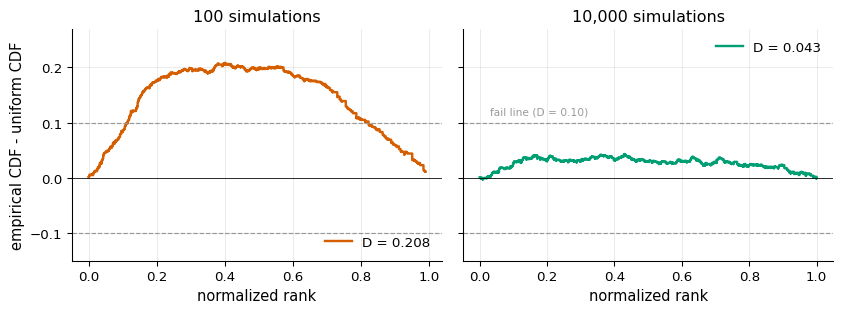
The undertrained fit arches well past the 0.10 fail line: its ranks concentrate away from uniform. The retrained fit settles onto the zero line, inside the fail band, which is what a calibrated likelihood looks like.
Warning
A lit check is a statement about this estimator on this data, not a verdict on the method. The SBC failure above says the 100-simulation fit is miscalibrated on the linear-Gaussian task, and more simulations resolved it. It says nothing general about NLE or MixedNLE. The discipline the docs teach is the loop: run the checks, and when one lights up, respond and re-check.
Note
Neural-likelihood approximation error has more effect on the posterior as more
observations enter a single inference, and there is no universal threshold for
when it matters. Validation reduces this risk but does not eliminate it: a
posterior predictive check (setu.posterior_predictive) is a useful
reference-free sanity check, though it cannot certify accuracy.
Where to go next#
Tutorial 1 runs the full Simulate → Train → Validate → Export workflow, including a validation pass, against an exact posterior. The glossary pins down SBC, C2ST, and the other diagnostics named here.