Modeling

To design a control system, it is first necessary to gain an understanding of how the system operates. This understanding is typically expressed in the form of a mathematical model which describes the steady state and dynamic behavior of the system.

In practice however, we can only derive a nominal model i.e. a mathematically simple and convenient system that is ideally close to the real system’s model. The latter differs from our nominal model because it can have different values of the parameters (parametric uncertainties) or some unmodelled dynamics, e.g., the senor’s inertia. These uncertainties are what explains the differences that exist between our designed controller’s results in a simulation and in the actual environment.

Modeling Approaches

Fig. 5 Illustration of different modeling approaches [DuunHenriksenSRoge+13]

• White box: The model is obtained based on physical equations. A deeper knowledge of the system is usually required.

• Black box: The model is identified based only on experimental data, without the use of prior knowledge.

• Grey box: Combines both approaches to relax the need to exactly model the underlying physics, while requiring considerably less data than a pure black box approach.

Notation

• Time:

  • Continuous-time: \(t \in \mathbb{R}\)

  • Discrete-time: \(t \in \mathbb{N}\)

• State:

  • Continuous-time: \(x(t) \in \mathbb{R}^n\)

  • Discrete-time: \(x_t \in \mathbb{R}^n\)

• Control input: \(u(t) \in \mathbb{R}^m\)

  • Continuous-time: \(u(t) \in \mathbb{R}^m\)

  • Discrete-time: \(u_t \in \mathbb{R}^m\)

• Dynamics

  • Continuous-time: \(\dot{x}(t) = f(x(t), u(t))\)

  • Discrete-time: \(x_{t+1} = f(x_t, u_t)\)

• Trajectories:

  • Continuous-time:

    • \(x: t \rightarrow x(t)\)

    • \(u: t \rightarrow u(t)\)

  • Discrete-time:

    • \(x: t \rightarrow x_t\)

    • \(u: t \rightarrow u_t\)

System Representation

• Transfer Function

• State-Space

• Input-Output

Transfer Function Representation

A transfer function of a system, sub-system, or component is a mathematical function that models the system’s output for each possible input.

Transfer functions are commonly used in the analysis of systems such as single-input single-output filters in the fields of signal processing, communication theory, and control theory. The term is often used exclusively to refer to linear time-invariant (LTI) systems. Most real systems have non-linear input/output characteristics, but many systems, when operated within nominal parameters have behavior close enough to linear that LTI system theory is an acceptable representation of the input/output behavior.

For continuous-time input signal \(x(t)\) and output \(y(t)\), dividing the Laplace transform of the output, \(\mathbf{Y}(s) = \mathcal{L}\left\{y(t)\right\}\), by the Laplace transform of the input, \(\mathbf{X}(s) = \mathcal{L}\left\{x(t)\right\}\), yields the system’s transfer function \(\mathbf{G}(s)\):

\[ \mathbf{G}(s) = \frac{\mathbf{Y}(s)}{\mathbf{X}(s)} = \frac{ \mathcal{L}\left\{y(t)\right\} }{ \mathcal{L}\left\{x(t)\right\}} \]

Where \(s = \sigma + j \cdot \omega\) is a complex variable. When we’re only interested in the steady-state response of the system then it is sufficient to set \(\sigma = 0\) (thus \(s = j \cdot \omega\)), which reduces the Laplace transforms with complex arguments to Fourier transforms with real argument \(\omega\).

The transfer function was the primary tool used in classical control engineering. However, it has proven to be unwieldy for the analysis of multiple-input multiple-output (MIMO) systems, and has been largely supplanted by state space representations for such systems. In spite of this, a transfer matrix can always be obtained for any linear system, in order to analyze its dynamics and other properties: each element of a transfer matrix is a transfer function relating a particular input variable to an output variable.

The transfer function has the general form:

\[ \mathbf{G}(s) = K \frac{(s - a_1)(s - a_2)\dots}{(s - b_1)(s - b_2)(s - b_3)\dots} \]

Where:

• \(K\) is the system’s gain.

• \(a_i\) are the system’s zeros.

• \(b_i\) are the system’s poles.

Poles (respectively Zeros) of a transfer function are the frequencies for which the value of the denominator (respectively numerator) becomes infinite (respectively zero). The values of the poles and the zeros of a system determine whether the system is stable, and how well the system performs. Control systems, in the most simple sense, can be designed simply by assigning specific values to the poles and zeros of the system.

Physically realizable control systems must have a number of poles greater than the number of zeros. Systems that satisfy this relationship are called Proper.

Laplace Transform

The Laplace transform is an integral transform that converts a function of a real variable (usually \(t\), in the time domain) to a function of a complex variable \(s\).

The Laplace transform of a function \(f(t)\), defined for all real numbers \(t \ge 0\), is the function \(F(s)\), which is a unilateral transform defined by:

\(F(s) = \mathcal{L}\left\{f(t)\right\} = \int\limits_{0}^{\infty} f(t)e^{-st}dt\)

where \(s\) is a complex frequency domain parameter \(s=\sigma +i\omega\), with real numbers \(\sigma\) and \(\omega\).

The inverse Laplace transform is defined as:

\(\mathcal{L}^{-1}\left\{F(s)\right\} = f(t)\)

Some of the Laplace transform’s properties include:

• One-to-One

  \[\mathcal{L}\left\{f(t)\right\} = \mathcal{L}\left\{g(t)\right\}, \text{ if and only if } f(t) = g(t)\]

• Linearity

  \[\mathcal{L}(\alpha f(t) + \beta g(t)) = \alpha \mathcal{L}\left\{f(t)\right\} + \beta \mathcal{L}\left\{g(t)\right\} = \alpha F(s) + \beta G(s)\]

• Time Scaling

  \[\mathcal{L}\left\{f(at)\right\} = \frac{1}{a} F(\frac{s}{a}), \text{ where } a \gt 0\]

• Frequency Shifting

  \[\mathcal{L}\left\{e^{at}f(t)\right\} = F(s - a), \text{ where } a \gt 0\]

• Derivative

  \[\mathcal{L}\left\{\frac{d f(t)}{dt}\right\} = s F(s) - f(0)\]

  For higher-order derivatives:

  \[\mathcal{L}\left\{\frac{d^n f(t)}{dt^n}\right\} = s^n F(s) - s^{n-1} f(0) - s^{n-2} \frac{d f(t)}{dt}|_{t=0} - \dots - \frac{d^{n-1} f(t)}{dt^{n-1}}|_{t=0}\]

The following is a list of Laplace transforms for common functions:

• Unit Step

  \[\mathcal{L}\left\{u(t)\right\} = \frac{1}{s}\]

  Where \(u(t) = 1, \text{ for } t \ge 0\).

• Unit Impulse

  \[\mathcal{L}\left\{\delta(t)\right\} = 1\]

  Where \(\delta(t) = \begin{cases}1, \text{ for } t = 0\\0, \text{ for } t \gt 0\end{cases}\)

• Exponential Decay

  \[\mathcal{L}\left\{e^{-\alpha t}u(t)\right\} = \frac{1}{s+\alpha}\]

  Where \(u(t)\) is the unit step function.

Exercise 2 (RC-Circuit Exercise)

Given the following RC circuit with an external voltage source:

Fig. 6 Schematic created using CircuitLab

The differential equation governing the charge of capacitor is given by:

\[\frac{d y(t)}{dt} + y(t) = u(t)\]

with:

• \(y(0) = 0\) i.e. the capacitor is uncharged at \(t=0\)

• \(u(t) = 1, \text{ for } t \ge 0\) i.e. the unit step.

Find the Laplace transform of the capacitor charge and then use it to solve the differential equation.

Solution to ( 2

\[\mathcal{L}\left\{\frac{d y(t)}{dt}\right\} + \mathcal{L}\left\{y(t)\right\} = \mathcal{L}\left\{u(t)\right\}\]

Applying the properties describe above we obtain:

\[s Y(s) + Y(s) = \frac{1}{s}\]

Rearranging we obtain:

\[Y(s) = \frac{1}{s(s+1)} = \frac{1}{s} - \frac{1}{s+1}\]

Finally, using the inverse Laplace transform we obtain:

\[y(t) = \mathcal{L}^{-1}\left\{Y(s)\right\} = 1 - e^{-t}\]

Closed-loop Transfer Function

Fig. 7 Closed Loop Block Dia

The transfer function of this system is given by:

\[ {\dfrac {Y(s)}{X(s)}}={\dfrac {G(s)}{1+G(s)H(s)}} \]

\(\displaystyle G(s)\) is called feedforward transfer function, \(\displaystyle H(s)\) is called feedback transfer function, and their product \(G(s)H(s)\) is called the open-loop transfer function.

State-Space Representation

A state-space representation is a mathematical model of a physical system specified as a set of input, output and variables related by first-order (not involving second derivatives) differential equations or difference equations.

Such variables, called state variables, evolve over time in a way that depends on the values they have at any given instant and on the externally imposed values of input variables. Output variables’ values depend on the values of the state variables.

Continuous-time Systems

\[\begin{split} \dot{\mathbf{x}}(t) = f(x(t), u(t)) \\ \mathbf{y}(t) = g(x(t), u(t)) \end{split}\]

Discrete-time Systems

\[\begin{split} \mathbf{x}_{t+1} = f(x_t, u_t) \\ \mathbf{y}_{k+1} = g(x_t, u_t) \end{split}\]

Table 1 State-Space Representation Forms Wikipedia

System type	State-space model
Continuous time-invariant	$\(\begin{align*}\dot{\mathbf{x}}(t) = A \mathbf{x}(t) + B \mathbf{u} (t)\\ \mathbf{y}(t) = C \mathbf{x}(t) + D \mathbf{u}(t)\end{align*}\)$
Continuous time-variant	$\(\begin{align*}\dot{\mathbf{x}}(t) = A(t) \mathbf{x}(t) + B(t) \mathbf{u}(t) \\ \mathbf{y}(t) = C(t) \mathbf{x}(t) + D(t) \mathbf{u}(t) \end{align*}\)$
Discrete time-invariant	$\(\begin{align*} \mathbf{x}(k+1) = A \mathbf{x}(k) + B \mathbf{u}(k) \\ \mathbf{y}(k+1) = C \mathbf{x}(k) + D \mathbf{u}(k) \end{align*}\)$
Discrete time-variant	$\(\begin{align*} \mathbf{x}(k+1) = A(k) \mathbf{x}(k) + B(k) \mathbf{u}(k) \\ \mathbf{y}(k+1) = C(k) \mathbf{x}(k) + D(k) \mathbf{u}(k) \end{align*}\)$
Laplace domain of continuous time-invariant	$\(\begin{align*}s\mathbf{X}(s) - \mathbf{x}(0) = A \mathbf{X}(s) + B \mathbf{U}(s) \\ \mathbf{Y}(s) = C \mathbf{X}(s) + D \mathbf{U}(s)\end{align*}\)$
Z-domain of discrete time-invariant	$\(\begin{align*}z\mathbf{X}(z) - z\mathbf{x}(0) = A \mathbf{X}(z) + B \mathbf{U}(z) \\ \mathbf{Y}(z) = C \mathbf{X}(z) + D \mathbf{U}(z)\end{align*}\)$

From State-Space to Transfer Function

\[\begin{split} \dot{\mathbf{x}}(t)= A \mathbf{x}(t) + B \mathbf{u}(t)\\ \mathbf{y}(t) = C \mathbf{x}(t) + D \mathbf{u}(t) \end{split}\]

We take the Laplace Transform (assuming X(0) = 0):

\[\begin{split} s{\mathbf{X}}(s)= A \mathbf{X}(s) + B \mathbf{U}(s)\\ \mathbf{Y}(s) = C \mathbf{X}(s) + D \mathbf{U}(s) \end{split}\]

We want to solve for \(\mathbf{G}(s) = \frac{{\mathbf{Y}}(s)}{\mathbf{U}(s)}\), so we start by solving for \({\mathbf{X}}(s)\):

\[ {\mathbf{X}}(s) = (sI - A)^{-1}B \mathbf{U}(s) \]

Now we put this into the output equation:

\[ {\mathbf{Y}}(s) = \left(C(sI - A)^{-1}B + D\right) \mathbf {U}(s) \]

\[ \mathbf{G}(s) = \frac{{\mathbf{Y}}(s)}{\mathbf{U}(s)} = C(sI - A)^{-1}B + D \]

Input-Output Representation

For some systems, it may be difficult, or sometimes impossible, to obtain a mathematical dynamical model from physical laws. In that case, one can try to describe the dynamical behavior through so-called input-output relations.

Continous-time Systems

\[ \frac{d^{n}{\mathbf{y}(t)}}{dt^{n}} = \mathbf{h}(\frac{d^{n-1}{\mathbf{y}(t)}}{dt^{n-1}}, \frac{d^{n-2}{\mathbf{y}(t)}}{dt^{n-2}}, \dots, \mathbf{u}(t), \frac{d{\mathbf{u}(t)}}{dt}, \dots) \]

Discrete-time Systems

\[ \mathbf{y}_t = \mathbf{h}(\mathbf{y}_{t-1}, \mathbf{y}_{t-2}, \dots, \mathbf{u}_t, \mathbf{u}_{t-1}, \dots) \]

This representations is mostly used in black-box modeling for identifying system dynamics without any prior knowledge.

Inverted Pendulum Model

Fig. 8 Inverted pendulum model [Goo00]

• \(y(t)\): distance along the horizontal axis from some reference point.

• \(\theta(t)\): angle of the pendulum.

• \(M\): mass of the cart.

• \(m\): mass of the pendulum (assumed to be concentrated at the tip).

• \(l\): length of the pendulum.

• \(f(t)\): force applied on the cart.

Application of Newtonian physics to this system leads to the following model:

\[\begin{split} \ddot{y}(t) = \frac{1}{m\cos^2\theta(t) - (1+k)(M+m)} \left[ mg\sin\theta(t)\cos\theta(t) - (1+k)(f(t) + ml\dot\theta^2(t) \sin\theta(t)) \right]\\ \ddot\theta(t) = \frac{1}{(1+k)(M+m)l - ml\cos^2\theta(t)} \left[ (M+m)g\sin\theta(t) - \cos\theta(t) (f(t) + ml\dot\theta^2(t)\sin\theta(t)) \right] \end{split}\]

with \(k = \frac{1}{3}.\)

We’re only interested in controlling the pendulum’s angle, so we can ignore the first equation.

We can convert this to state space form with input \(u(t) = f(t)\) and output \(y(t)\); by introducing:

\[\begin{split} X(t) = \begin{bmatrix} x_1(t) \\ x_2(t) \end{bmatrix} = \begin{bmatrix} \theta(t) \\ \dot{\theta}(t) \end{bmatrix} \end{split}\]

\[\begin{split} \dot{X}(t) = \begin{bmatrix} \dot{x}_1(t) \\ \dot{x}_2(t) \end{bmatrix} = \begin{bmatrix} x_2(t) \\ \frac{1}{(1+k)(M+m)l - ml\cos^2 x_1(t)} \left[ (M+m)g\sin x_1(t) - \cos x_1(t) (u(t) + ml x_2^2(t)\sin x_1(t))\right] \\ \end{bmatrix} \end{split}\]

These equations are nonlinear. However, for small departures of \(x_1\) (i.e. \(\theta\)) from the vertical position we can linearize about \(x_1 = 0\), \(x_2 = 0\). This is called the small-angle approximation.

Exercise 3 (Small Angle Approximation Exercise)

• How good is the small angle approximation?

Solution to ( 3

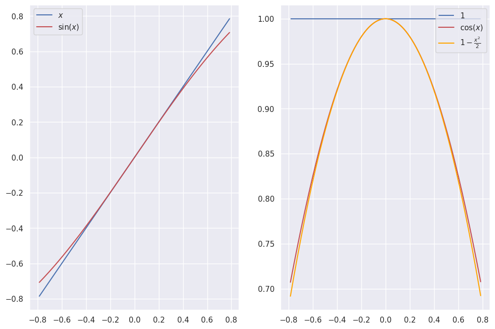
Applying the approximation gives us:

\[\begin{split} \dot{X}(t) = \begin{bmatrix} \dot{x}_1(t) \\ \dot{x}_2(t) \end{bmatrix} = \begin{bmatrix} x_2(t) \\ \frac{1}{M l} \left[ - \gamma u(t) + (M + m) g x_1(t) \right] \\ \end{bmatrix} = \begin{bmatrix} 0 & 1\\ \frac{(M + m)g}{Ml} & 0\\ \end{bmatrix} \begin{bmatrix} x_1(t) \\ x_2(t) \end{bmatrix} + \begin{bmatrix} 0 \\ -\frac{1}{Ml} \end{bmatrix} \begin{bmatrix} u(t)\\ \end{bmatrix} \end{split}\]

This leads to a linear state-space model with matrices:

\[\begin{split} A = \begin{bmatrix} 0 & 1 \\ \frac{(M + m)g}{Ml} & 0\\ \end{bmatrix}; B = \begin{bmatrix} 0 \\ -\frac{1}{Ml} \end{bmatrix}; C = \begin{bmatrix} 1 & 0 \\ \end{bmatrix}; D = \begin{bmatrix} 0 \end{bmatrix} \end{split}\]

And this the corresponding transfer function:

\[\begin{split} (sI - A)^{-1} = \begin{bmatrix} s & - 1 \\ - \frac{(M + m)g}{Ml} & s\\ \end{bmatrix}^{-1} = \frac{1}{Mls^2 - g(M+m)} \begin{bmatrix} Mls & Ml \\ g(M+m) & Mls\\ \end{bmatrix} \end{split}\]

\[ \mathbf{G}(s) = C(sI - A)^{-1}B + D = \frac{-1}{Mls^2 - g(M+m)} \]

System Identification

System Identification is the process of constructing a mathematical model of a (dynamical) system from observations (measurements) of its inputs and outputs. It uses statistical methods to build mathematical models of dynamical systems from measured data. System identification also includes the optimal design of experiments for efficiently generating informative data for fitting such models as well as model reduction.

In control engineering, the objective is to obtain a good performance of the closed-loop system, which is the one comprising the physical system, the feedback loop and the controller. This performance is typically achieved by designing the control law relying on a model of the system, which needs to be identified starting from experimental data. If the model identification procedure is aimed at control purposes, what really matters is not to obtain the best possible model that fits the data, as in the classical system identification approach, but to obtain a model satisfying enough for the closed-loop performance.

Structural Identifiability

In structural identifiability, given a model for a given system, we would like to know whether the unknown parameters are uniquely determined by the input-output behaviour of the system.

In certain cases, the model structure may not permit a unique solution for this estimation problem, even when the data is continuous and free from noise. To avoid potential issues, it is recommended to verify the uniqueness of the solution in advance, prior to conducting any actual experiments. The lack of structural identifiability implies that there are multiple solutions for the problem of system identification, and the impossibility of distinguishing between these solutions suggests that the system has poor forecasting power as a model.

Consider an LTI system with the following state-space representation:

\[\begin{split} \displaystyle {\begin{aligned} {\dot{\mathbf{x}}}_{1}(t) &= -\theta _{1}\mathbf{x}_{1}\\ {\dot {\mathbf{x}}}_{2}(t) &= \theta _{1}\mathbf{x}_{1}\\ \mathbf{y}(t) &=\theta _{2}\mathbf{x}_{2} \end{aligned}} \end{split}\]

and with initial conditions given by \(\displaystyle \mathbf{x}_{1}(0)=\theta_{3}\) and \(\displaystyle \mathbf{x}_{2}(0) = 0\). The solution of the output \(\mathbf{y}\) is

\[ \displaystyle \mathbf{y}(t) = \theta_{2}\theta_{3}e^{-\theta_{1}t}\left(e^{\theta_{1}t}-1\right), \]

which implies that the parameters \(\theta_2\) and \(\displaystyle \theta_{3}\) are not structurally identifiable. For instance, the parameters \(\displaystyle \theta _{1}=1,\theta _{2}=1,\theta _{3}=1\) generate the same output as the parameters \(\displaystyle \theta _{1}=1,\theta _{2}=2,\theta _{3}=0.5\).

Exercise 4 (Inverted Pendulum Parameter Identifiability)

• Which parameters of the inverted pendulum system are identifiable and which ones are not?

Parameter Identification

Parameter identification or parameter estimation deals with estimating the values of parameters based on measured empirical data that has a random component. The parameters describe an underlying physical setting in such a way that their value affects the distribution of the measured data. An estimation method attempts to approximate the unknown parameters using the measurements.

Commonly used estimation methods include:

• Eigensystem Realization algorithm (ERA)

• Proper Orthogonal Decomposition (POD)

• Balanced POD (BPOD)

• Maximum likelihood estimators

• Least squares

• Minimum mean squared error (MMSE), also known as Bayes least squared error (BLSE)

• Maximum a posteriori (MAP)

• Particle filter

• Kalman filter, and its various derivatives

Second Order Resonant System

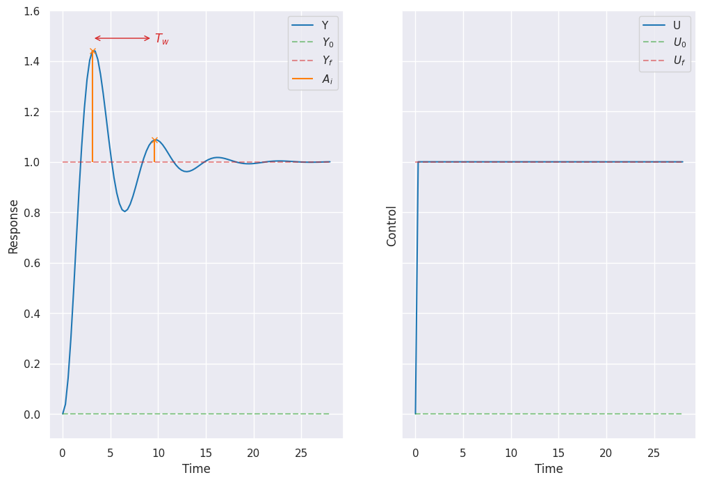
• \(U_0\): Initial input level.

• \(U_f\): Final input level.

• \(Y_0\): Initial output level.

• \(Y_f\) : Final output level.

• Peak 1: First output peak.

• Peak n: Peak n counting from Peak 1.

• \(A_1\): Amplitude from \(Y_f\) to Peak 1.

• \(A_n\): Amplitude from \(Y_f\) to Peak n.

• \(T_w\) : Time between two successive peaks.

Given those measurements we can calculate the system’s parameters using:

\[\begin{split} K = \frac{Y_f - Y_0}{U_f - U_0}\\ d_r =\left(\frac{A_n}{A_1}\right)^{\frac{1}{n−1}}\\ \hat{\zeta} = -\frac{\ln(d_r)}{\sqrt{4\pi^2 + \sqrt{d_r}^2}}\\ \hat{T_n} = \frac{T_w \sqrt{1 - \hat{\zeta}^2}}{2\pi} \end{split}\]

And then plug their values into the following transfer function:

\[ \hat{G}(s) = \frac{\hat{K}}{\hat{T_n}^2 s^2 + 2\hat{\zeta}\hat{T}_n s + 1} \]

Exercise 5 (Inverted Pendulum Parameter Identification)

• Identify the parameters of the Inverted Pendulum system using the method described above.

Tip

Hint What is the step response of the inverted pendulum?

Solution to ( 5

env = create_inverted_pendulum_environment()
l = env.length
m = env.masspole
M = env.masscart
g = env.gravity
print(f"{l=}, {m}, {M=}, {g=}")

l=1.0, 0.1, M=1.0, g=9.81

# Dynamics matrix
A = np.array(
    [
        [0, 1],
        [(M + m) * g / (M * l), 0],
    ]
)
# Input matrix
B = np.array([[0, -1 / (M * l)]]).transpose()
# Output matrices
C = np.array(
    [
        [1, 0],
    ]
)
D = np.zeros(1)

inverted_pendulum = ct.ss(A, B, C, D)
inverted_pendulum.name = "inverted_pendulum"
inverted_pendulum

\[\begin{split} \left(\begin{array}{rllrll|rll} 0\phantom{.}&\hspace{-1em}&\hspace{-1em}\phantom{\cdot}&1\phantom{.}&\hspace{-1em}&\hspace{-1em}\phantom{\cdot}&0\phantom{.}&\hspace{-1em}&\hspace{-1em}\phantom{\cdot}\\ 10.&\hspace{-1em}8&\hspace{-1em}\phantom{\cdot}&0\phantom{.}&\hspace{-1em}&\hspace{-1em}\phantom{\cdot}&-1\phantom{.}&\hspace{-1em}&\hspace{-1em}\phantom{\cdot}\\ \hline 1\phantom{.}&\hspace{-1em}&\hspace{-1em}\phantom{\cdot}&0\phantom{.}&\hspace{-1em}&\hspace{-1em}\phantom{\cdot}&0\phantom{.}&\hspace{-1em}&\hspace{-1em}\phantom{\cdot}\\ \end{array}\right) \end{split}\]

tf = ct.ss2tf(inverted_pendulum)
tf

\[\frac{-4.441 \times 10^{-16} s - 1}{s^2 - 10.79}\]

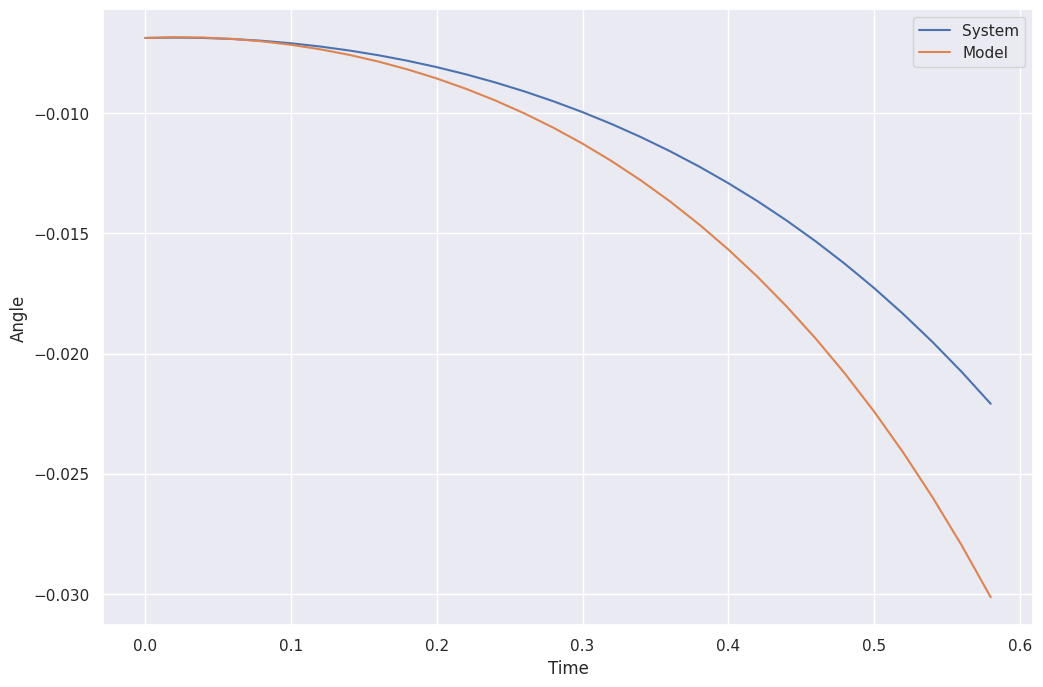
We can now compare our model with observations from the actual environment.

max_steps = 30
env = create_inverted_pendulum_environment(max_steps=max_steps)
controller = ConstantController()
results = simulate_environment(env, max_steps=max_steps, controller=controller)

error: XDG_RUNTIME_DIR not set in the environment.

dt = env.dt
T = np.arange(len(results.observations)) * env.dt
T = T[:-1]
U = results.actions.transpose()
X0 = results.observations[0, [2, 3]]
response = ct.input_output_response(inverted_pendulum, T, U, X0)

plt.plot(response.time, response.outputs, label="System")
plt.plot(response.time, results.observations[:-1, 2], label="Model")
plt.xlabel("Time")
plt.ylabel("Angle")
plt.legend();

Stability

There are many notions of stability in Control Theory:

• BIBO Stability

  A system is bounded-input, bounded-output stable (BIBO stable) if, for every bounded input, the output is finite. Mathematically, if every input satisfying

  \[ ||u(t)||_\infty \lt \infty \]

  leads to an output satisfying

  \[ ||y(t)||_\infty \lt \infty \]

• Marginal/Lyapunov \(\forall \epsilon > 0, \exists \delta > 0 : ||x(0) - x_{\text{eq}}|| < \delta \implies ||x(t) - x_{\text{eq}}|| < \epsilon, \forall t \gt 0\)

  Trajectories that start close to the equilibrium remain close to the equilibrium.

• Asymptotic (local) \(\exists \delta > 0 : ||x(0) - x_{\text{eq}}|| < \delta \implies \lim_{\rightarrow \infty} ||x(t) - x_{\text{eq}}|| = 0\)

  Trajectories that start near the equilibrium converge to it.

• Exponential (local) \(\exists \delta, c, \alpha > 0 : ||x(0) − x_{\text{eq}}|| < \delta \implies ||x(t) - x_{\text{eq}}|| \lt c\exp^{−\alpha t} || x(0) - x_{\text{eq}}||\)

  Trajectories that start near the equilibrium converge to it exponentially fast.

Note

The global definitions can be obtained by taking \(\delta \rightarrow \infty\).

Note

For linear time-invariant (LTI) systems, “asymptotic = exponential” and “local = global” always.

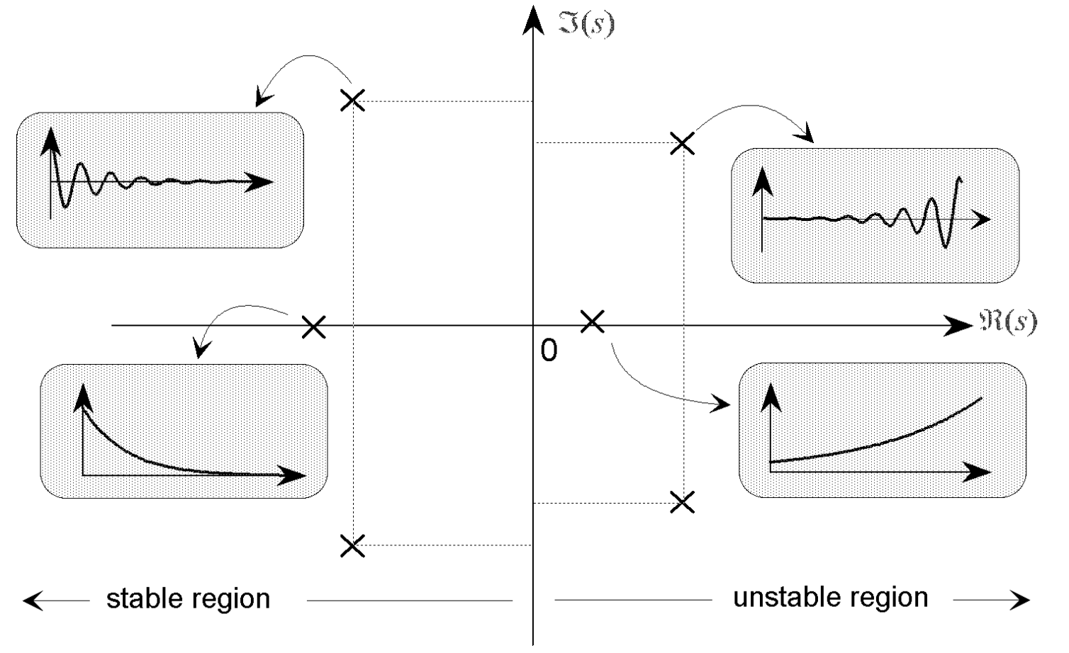
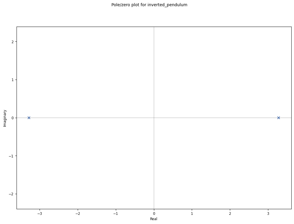
A Linearly Time-Invariant (LTI) system is stable if and only if:

• All the poles are in the left half of the complex plane (i.e. they have a negative real part).

• All the eigenvalues of \(A\) have negative real parts.

• We can find two \(p \times p\) matrices \(M\) and \(N\) such that satisfy the Lyapunov Equation:

  \[ MA + A^TM = -N \]

  and \(N\) is an arbitrary positive definite matrix, and \(M\) is a unique positive definite matrix.

LTI State-Transition Matrix

The solution to the following continous-time state-space model:

\[ \dot{\mathbf{x}}(t)= A \mathbf{x}(t) + B \mathbf {u} (t) \]

is given by:

\[ \mathbf{x}(t) = \Phi(t)\mathbf{x}(0) + \int\limits_{0}^{\infty} \Phi(t - \tau) B \mathbf{u}(\tau) d\tau \]

where: \(\Phi(t) = e^{At}\)

The unforced or homogeneous response (\(\mathbf{u}(t) = 0\)) of this system is:

\[ \mathbf{x}(t) = e^{At}\mathbf{x}(0) \]

which can be rewritten using the eigendecomposition as:

\[ \mathbf{x}(t) = \left[M e^{\Lambda t}M^{-1}\right] \mathbf{x}(0) \]

where

• \(e^{\Lambda t} = \begin{bmatrix} e^{\lambda_1 t} & 0 & \dots & 0 & 0\\ 0 & e^{\lambda_2 t} & 0 & \dots & 0 \\ 0 & 0 & \dots & \ddots & 0\\ 0 & 0 & \dots & 0 & e^{\lambda_n t}\\ \end{bmatrix}\)

• \(\Lambda\) is a vector that contains the eigenvalues of \(A\).

• \(M = \begin{bmatrix}m_{ij}\end{bmatrix}\) is a matrix whose columns are the eigenvectors of \(A\).

Exercise 6 (State-Transition Matrix exercise)

Determine state-transition matrix for an LTI system with the following dynamics matrix \(A\):

\[\begin{split} A = \begin{bmatrix} -2 & 1\\ 2 & -3 \end{bmatrix} \end{split}\]

1. Determine the eigenvalues and eigenvectors of the dynamics matrix.

2. Determine the state-transition matrix.

3. What can we say about the system’s stability given the initial conditions \(x_1(t) = 0, x_2(t) = 2\)

Tip

• use np.linalg.eig(A) to determine the eigenvalues and eigenvectors of a matrix \(A\).

• use np.linalg.inv(M) to compute the inverse of a matrix \(M\).

Solution to ( 6

A = np.array([[-2, 1], [2, -3]])
Lambda, M = np.linalg.eig(A)
M_1 = np.linalg.inv(M)
t = sym.symbols("t")
phi = M * sym.simplify(sym.exp(sym.Matrix(np.diag(Lambda) * t))) * M_1
x0 = np.array([[0], [2]])
x = phi * x0
display_array("A", A)
display_array("\Lambda", Lambda)
display_array("M", M)
display_array("M^{-1}", M_1)
display_array("\Phi(t)", phi)
display_array("x(t)", x)

\[\begin{split}\displaystyle \begin{equation*}A = \begin{bmatrix}-2 &1 \\2 &-3 \\\end{bmatrix}\end{equation*}\end{split}\]

\[\begin{split}\displaystyle \begin{equation*}\Lambda = \begin{bmatrix}-1.0 \\-4.0 \\\end{bmatrix}\end{equation*}\end{split}\]

\[\begin{split}\displaystyle \begin{equation*}M = \begin{bmatrix}0.7071067811865475 &-0.4472135954999579 \\0.7071067811865475 &0.8944271909999159 \\\end{bmatrix}\end{equation*}\end{split}\]

\[\begin{split}\displaystyle \begin{equation*}M^{-1} = \begin{bmatrix}0.9428090415820636 &0.4714045207910317 \\-0.7453559924999299 &0.7453559924999299 \\\end{bmatrix}\end{equation*}\end{split}\]

\[\begin{split}\displaystyle \begin{equation*}\Phi(t) = \begin{bmatrix}0.333333333333333*exp(-4.0*t) + 0.666666666666667*exp(-t) \\-0.333333333333333*exp(-4.0*t) + 0.333333333333333*exp(-t) \\-0.666666666666667*exp(-4.0*t) + 0.666666666666667*exp(-t) \\0.666666666666667*exp(-4.0*t) + 0.333333333333333*exp(-t) \\\end{bmatrix}\end{equation*}\end{split}\]

\[\begin{split}\displaystyle \begin{equation*}x(t) = \begin{bmatrix}-0.666666666666667*exp(-4.0*t) + 0.666666666666667*exp(-t) \\1.33333333333333*exp(-4.0*t) + 0.666666666666667*exp(-t) \\\end{bmatrix}\end{equation*}\end{split}\]

Note

The system’s response is composed of two decaying exponentials which means that system is asymptotically stable with stable end-state \(x(\infty) = \begin{bmatrix} 0 \\ 0\end{bmatrix}\)

Exercise 7 (Linearized Model Stability)

Determine whether the linearized inverted pendulum system is stable.

Tip

• Use the poles() method of the inverted_pendulum object to determine the system’s poles.

• Use np.linalg.eig to determine the eigenvalues of the system matrix.

• Use ct.lyap to solve the lyapunov equation.

Solution to ( 7

poles = inverted_pendulum.poles()
poles
print(f"Is the real part of all poles negatives? {np.all(np.real(poles) <= 0.0)}")
print("This means that the system is unstable.")

Is the real part of all poles negatives? False
This means that the system is unstable.

For the sake of demonstration, let’s also compute the system matrix’ eigenvalues and compare them to the poles

eigenvalues, _ = np.linalg.eig(inverted_pendulum.A)
eigenvalues
print(f"Are the eigenvalues equal to the poles? {np.all(poles == eigenvalues)}")

Are the eigenvalues equal to the poles? True

We can visualize the system’s poles and zeros

ct.pzmap(inverted_pendulum);

Observability

Observability is a measure for how well internal states of a system can be inferred by knowledge of its external outputs..

For a continuous linear time-invariant system, the \(n \times nr\) observability matrix is given by:

\(O=\begin{bmatrix}C \\ CA \\ CA^{2} \\ \dots \\ CA^{n-1}\end{bmatrix}\)

The system is controllable if the observability matrix has full row rank (i.e. \(\operatorname{rank}(O)=n\)).

O = ct.obsv(inverted_pendulum.A, inverted_pendulum.C)
print(O)

[[1. 0.]
 [0. 1.]]

np.linalg.matrix_rank(O)

2

This means that the system is observable.

Parameter Estimation using an Observer

Consider the augmented state vector \(\mathbf{z}(t)\):

\[\begin{split} \mathbf{z}(t) = \begin{bmatrix} \mathbf{x}(t) \\ \mathbf{p} \end{bmatrix} \end{split}\]

Where \(\mathbf{p}\) represents the system’s parameters.

This new system has the following dynamics:

\[\begin{split} \dot{\mathbf{z}}(t) = \begin{bmatrix} \dot{\mathbf{x}}(t) \\ \dot{\mathbf{p}} \end{bmatrix} = \begin{bmatrix} A\mathbf{x}(t) + B\mathbf{u}(t) \\ 0 \end{bmatrix} \end{split}\]

If this system is observable then we can use an observer to estimate the system’s parameters. Unfortunately, this system is no longer linear and thus requires a different approach.

Observer Design

Kalman Filter

Kalman filtering, also known as linear quadratic estimation (LQE), is an algorithm that uses a series of measurements observed over time, including statistical noise and other inaccuracies, and produces estimates of unknown variables that tend to be more accurate than those based on a single measurement alone, by estimating a joint probability distribution over the variables for each timeframe.

The Kalman filter model assumes the true state at time \(t\) is described by a linear state-space model:

\[\begin{split} \mathbf{x}_{t+1} = A_t\mathbf{x}_t + B_t\mathbf{u}_t + \mathbf{w}_t\\ \end{split}\]

at time \(t\) an observation (or measurement) \(\mathbf{z}_t\) of the true state \(\mathbf{x}_t\) is made according to

\[ \mathbf{z}_t = H_t \mathbf{x}_t + \mathbf{v}_t \]

Where:

• \(\mathbf{w}_t\) is the process noise, which is assumed to be drawn from a zero-mean multivariate normal distribution, \(\mathcal{N}\), with covariance, \(\mathbf{w}_{t} \sim {\mathcal {N}}\left(0,\mathbf {Q} _{t}\right)\).

• \(\mathbf{v}_t\) is the observation noise, which is assumed to be zero-mean Gaussian white noise with covariance \(\mathbf{v} _{t}\sim {\mathcal {N}}\left(0,\mathbf {R} _{t}\right)\).

• \(H_t\) is the observation model, which maps the true state space into the observed space and

Predict

• Predicted (a priori) state estimate: \(\displaystyle {\hat{\mathbf{x}}}_{t\mid t-1} = \mathbf{A}_{t}\mathbf{x}_{t-1\mid t-1}+\mathbf{B}_{t}\mathbf{u}_{t-1}\)

• Predicted (a priori) estimate covariance: \(\displaystyle {\hat{\mathbf{P}}}_{t\mid t-1} = \mathbf{A}_{t} \mathbf{P}_{t-1\mid t-1}\mathbf{A}_{t}^{\textsf{T}} + \mathbf{Q}_{t}\)

Update

• Innovation or measurement pre-fit residual: \(\displaystyle {\tilde {\mathbf {y}}}_{t} = \mathbf {z}_{t}-\mathbf{H}_{t}{\hat {\mathbf{x}}}_{t\mid t-1}\)

• Innovation (or pre-fit residual) covariance: \(\displaystyle \mathbf {S} _{t+1}=\mathbf {H} _{t+1}{\hat {\mathbf {P} }}_{t+1\mid t}\mathbf {H}_{t+1}^{\textsf {T}} + \mathbf {R}_{t+1}\)

• Optimal Kalman gain: \(\displaystyle \mathbf {K}_{t}={\hat{\mathbf{P}}}_{t\mid t-1}\mathbf{H}_{t}^{\textsf{T}}\mathbf{S}_{t}^{-1}\)

• Updated (a posteriori) state estimate: \(\displaystyle \mathbf{x}_{t\mid t} = {\hat{\mathbf{x}}}_{t\mid t-1} + \mathbf{K}_{t}{\tilde {\mathbf{y}}}_{t}\)

• Updated (a posteriori) estimate covariance: \(\displaystyle \mathbf{P}_{t|t} = \left(\mathbf{I} - \mathbf{K}_{t}\mathbf{H}_{t}\right){\hat{\mathbf{P}}}_{t|t-1}\)

• Measurement post-fit residual: \(\displaystyle {\tilde{\mathbf{y}}}_{t\mid t} = \mathbf{z}_{t} - \mathbf{H}_{t}\mathbf{x}_{t\mid t}\)

Fig. 9 Kalman Filter

Exercise 8 (Kalman Filter)

Design a Kalman Filter for the Inverted Pendulum system.

Solution to ( 8

We collect some data from the environment

max_steps = 50
env = create_inverted_pendulum_environment(max_steps=max_steps)
controller = ProportionalController(K=20)
results = simulate_environment(env, max_steps=max_steps, controller=controller)
observations = results.observations
actions = results.actions

Q = np.diag([10])
R = np.diag([1e-5])
# Initial State Covariance
P0 = np.diag([0.0, 100])
inverted_pendulum_estimator = ct.create_estimator_iosystem(
    inverted_pendulum, Q, R, P0=P0
)
inverted_pendulum_estimator.name = "estimator"
print(inverted_pendulum_estimator)

<NonlinearIOSystem>: estimator
Inputs (2): ['y[0]', 'u[0]']
Outputs (2): ['xhat[0]', 'xhat[1]']
States (6): ['xhat[0]', 'xhat[1]', 'P[0,0]', 'P[0,1]', 'P[1,0]', 'P[1,1]']

Update: <function create_estimator_iosystem.<locals>._estim_update at 0x7fda7c3b7ce0>
Output: <function create_estimator_iosystem.<locals>._estim_output at 0x7fda3c60eb60>

error: XDG_RUNTIME_DIR not set in the environment.

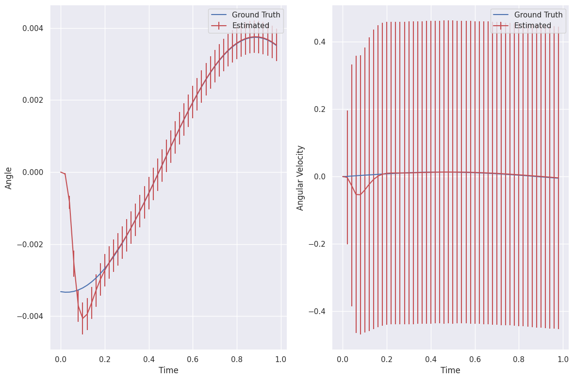
And run the estimator on the trajectory

env = create_inverted_pendulum_environment()
dt = env.dt
T = np.arange(0, len(observations) * dt, dt)
T = T[: len(observations) - 1]
U = np.concatenate([observations[1:, [2]], actions], axis=1).transpose()
X0 = np.zeros(2)
estimator_response = ct.input_output_response(inverted_pendulum_estimator, T, U, X0)

plot_estimator_response(
    estimator_response,
    labels=["Angle", "Angular Velocity"],
    observations=observations[:, [2, 3]],
)

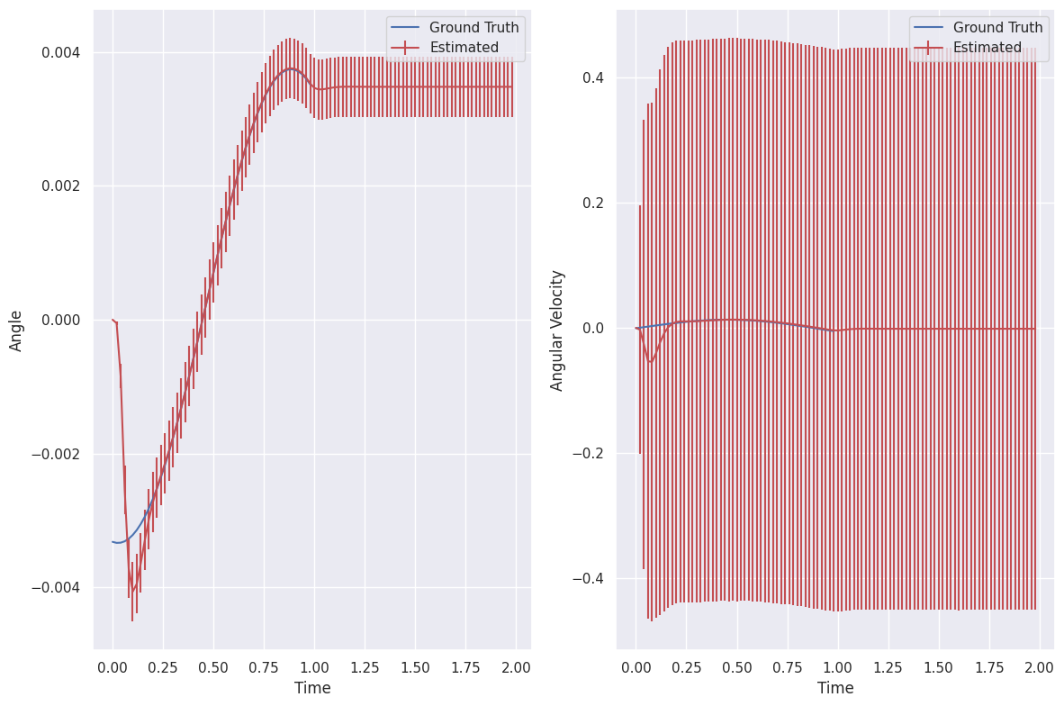
We also run predictions in the future to see what happens next

T_predict = np.arange(T[-1] + dt, T[-1] + 1.0 + dt, dt)
T = np.concatenate([T, T_predict])
U_predict = np.outer(U[:, -1], np.ones_like(T_predict))
U = np.concatenate([U, U_predict], axis=1)
predicted_response = ct.input_output_response(
    inverted_pendulum_estimator,
    T,
    U,
    X0,
)

plot_estimator_response(
    predicted_response,
    labels=["Angle", "Angular Velocity"],
    observations=observations[:, [2, 3]],
)

Controllability

The state controllability condition implies that it is possible - by admissible inputs - to steer the states from any initial value to any final value within some finite time window.

For a continuous linear time-invariant system, the \(n \times nr\) controllability matrix is given by:

\(R=\begin{bmatrix}B \\ AB \\ A^{2}B \\ \vdots \\ A^{n-1}B\end{bmatrix}\)

The system is controllable if the controllability matrix has full row rank (i.e. \(\operatorname{rank}(R)=n\)).

R = ct.ctrb(inverted_pendulum.A, inverted_pendulum.B)
print(R)

[[ 0. -1.]
 [-1.  0.]]

np.linalg.matrix_rank(R)

2

This means that the system is controllable.