Controller Design

Controller Design#

PID Controller#

Proportional–integral–derivative (PID) controller is a control loop mechanism employing feedback that is widely used in industrial control systems and a variety of other applications requiring continuously modulated control.

The overall control function:

\[ u(t) = K_{\text{P}}e(t) + K_{\text{I}}\int _{0}^{t}e(\tau )\,\mathrm {d} \tau + K_{\text{D}}{\frac {\mathrm {d} e(t)}{\mathrm {d} t}}, \]

where \(e(t) = y(t) - r(t)\), \(K_{\text{P}}\), \(K_{\text{I}}\), and \(K_{\text{D}}\), all non-negative, denote the coefficients for the proportional, integral, and derivative terms respectively.

The use of the PID algorithm does not guarantee optimal control of the system or its control stability but in practice it works really well for simple systems. It is broadly applicable since it relies only on the response of the measured process variable, not on knowledge or a model of the underlying process.

../_images/20_pid_block_diagram.svg — Fig. 10 PID Control Block Diagram#

The transfer function of the PID controller is given by:

\[ U(s) = K_P + \frac{K_I}{s} + K_D s = \frac{K_D s^2 + K_p s + K_I}{s} \]

This is not a proper transfer function (the number of zeros is higher than the number of poles). In order to make it proper, we modify the derivative term:

\[ K_D \frac{s}{\tau s + 1} \]

The PID controller’s transfer function then becomes:

\[ U(s) = K_P + \frac{K_I}{s} + K_D \frac{s}{\tau s + 1} = \frac{(K_D + \tau K_P) s^2 + (K_p + K_I \tau) s + K_I}{\tau s^2 + s} \]

PID Tuning#

There are several methods for tuning a PID loop. The most effective methods generally involve developing some form of process model and then choosing P, I, and D based on the dynamic model parameters. Manual tuning methods can be relatively time-consuming, particularly for systems with long loop times.

Table 2 PID Tuning Methods - Wikipedia#
Method	Advantages	Disadvantages
Manual Tuning	No mathematics required; online.	This is an iterative, experience-based, trial-and-error procedure that can be relatively time consuming. Operators may find “bad” parameters without proper training.
Ziegler–Nichols	Online tuning, with no tuning parameter therefore easy to deploy.	Process upsets may occur in the tuning, can yield very aggressive parameters. Does not work well with time-delay processes.
Tyreus Luyben	Online tuning, an extension of the Ziegler–Nichols method, that is generally less aggressive.	Process upsets may occur in the tuning; operator needs to select a parameter for the method which requires insight.
Cohen–Coon	Good process models.	Offline; only good for first-order processes.
Åström-Hägglund	Unlike the Ziegler–Nichols method this will not introduce a risk of loop instability. Little prior process knowledge required.	May give excessive derivative action and sluggish response. Later extensions resolve these issues, but require a more complex tuning procedure.
Simple control rule (SIMC)	Analytically derived, works on time delayed processes, has an additional tuning parameter that allows additional flexibility. Tuning can be performed with step-response model.	Offline method; cannot be applied to oscillatory processes. Operator must chose the additional tuning parameter.
Software tools	Consistent tuning; online or offline - can employ computer-automated control system design (CAutoD) techniques; may include valve and sensor analysis; allows simulation before downloading; can support non-steady-state (NSS) tuning.	“Black box tuning” that requires specification of an objective describing the optimal behaviour.

Manual tuning#

One of the many possible manual tuning methods follows these steps:

Set \(K_{I}\) and \(K_{D}\) values to zero.
Increase \(K_{P}\) until the output of the loop oscillates; then set \(K_{P}\) to approximately half that value for a “quarter amplitude decay”-type response (By “quarter wave decay” we mean that the transient response will (usually) decay four times faster).
Increase \(K_{I}\) until any offset is corrected in sufficient time for the process, but not until too great a value causes instability.
Finally, increase \(K_{D}\), if required, until the loop is acceptably quick to reach its reference after a load disturbance. Too much \(K_{D}\) causes excessive response and overshoot.

A fast PID loop tuning usually overshoots slightly to reach the reference more quickly; however, some systems cannot accept overshoot, in which case an overdamped closed-loop system is required, which in turn requires a \(K_{P}\) setting significantly less than half that of the \(K_{P}\) setting that was causing oscillation.

pid_controller = create_pid_controller(Kp=100, Ki=5, Kd=1)
pid_controller

\[\begin{split} \left(\begin{array}{rllrll|rll} -10\phantom{.}&\hspace{-1em}&\hspace{-1em}\phantom{\cdot}&-0\phantom{.}&\hspace{-1em}&\hspace{-1em}\phantom{\cdot}&1\phantom{.}&\hspace{-1em}&\hspace{-1em}\phantom{\cdot}\\ 1\phantom{.}&\hspace{-1em}&\hspace{-1em}\phantom{\cdot}&0\phantom{.}&\hspace{-1em}&\hspace{-1em}\phantom{\cdot}&0\phantom{.}&\hspace{-1em}&\hspace{-1em}\phantom{\cdot}\\ \hline -95\phantom{.}&\hspace{-1em}&\hspace{-1em}\phantom{\cdot}&50\phantom{.}&\hspace{-1em}&\hspace{-1em}\phantom{\cdot}&110\phantom{.}&\hspace{-1em}&\hspace{-1em}\phantom{\cdot}\\ \end{array}\right) \end{split}\]

Exercise 9 (PID Controller)

Find a combination of PID parameters for the Inverted Pendulum system.
Use a PID controller with those parameters to control the Inverted Pendulum environment.

Tip

Hint Use the training_classical_control.control.PIDController class.

Solution to ( 9

def tune_pid_inverted_pendulum(
    Kp=widgets.FloatSlider(min=0.0, max=1000.0, step=1, value=30.0),
    Ki=widgets.FloatSlider(min=0.0, max=100.0, step=1, value=1.0),
    Kd=widgets.FloatSlider(min=0.0, max=1000.0, step=1, value=10.0),
    tau=widgets.FloatSlider(min=0.001, max=1.0, step=0.1, value=0.1),
    theta0=widgets.FloatSlider(min=-0.05, max=0.05, step=0.01, value=0.01),
):
    n_steps = 300
    env = create_inverted_pendulum_environment()
    T = np.arange(0, n_steps) * env.dt
    x0 = np.zeros(2)
    x0[0] = theta0
    u0 = 0.0

    pid_controller = create_pid_controller(Kp=Kp, Ki=Ki, Kd=Kd, tau=tau)
    e_summer = ct.summing_junction(["-r", "y[0]"], "e")
    closed_loop = ct.interconnect(
        (inverted_pendulum, pid_controller, e_summer),
        inplist=["r"],
        outlist=["y[0]", "u[0]"],
    )

    response = ct.input_output_response(closed_loop, T, u0, x0)
    plot_inverted_pendulum_results(
        T, u0, response.states.transpose(), response.outputs[1, 1:]
    )


interact(tune_pid_inverted_pendulum);

Kp = 30
Ki = 1
Kd = 10

Evaluation

max_steps = 500
env = create_inverted_pendulum_environment(max_steps=max_steps)
r = 0.0
controller = PIDController(Kp=Kp, Ki=Ki, Kd=Kd, reference=r, dt=env.dt)
results = simulate_environment(env, max_steps=max_steps, controller=controller)
observations = results.observations
actions = results.actions
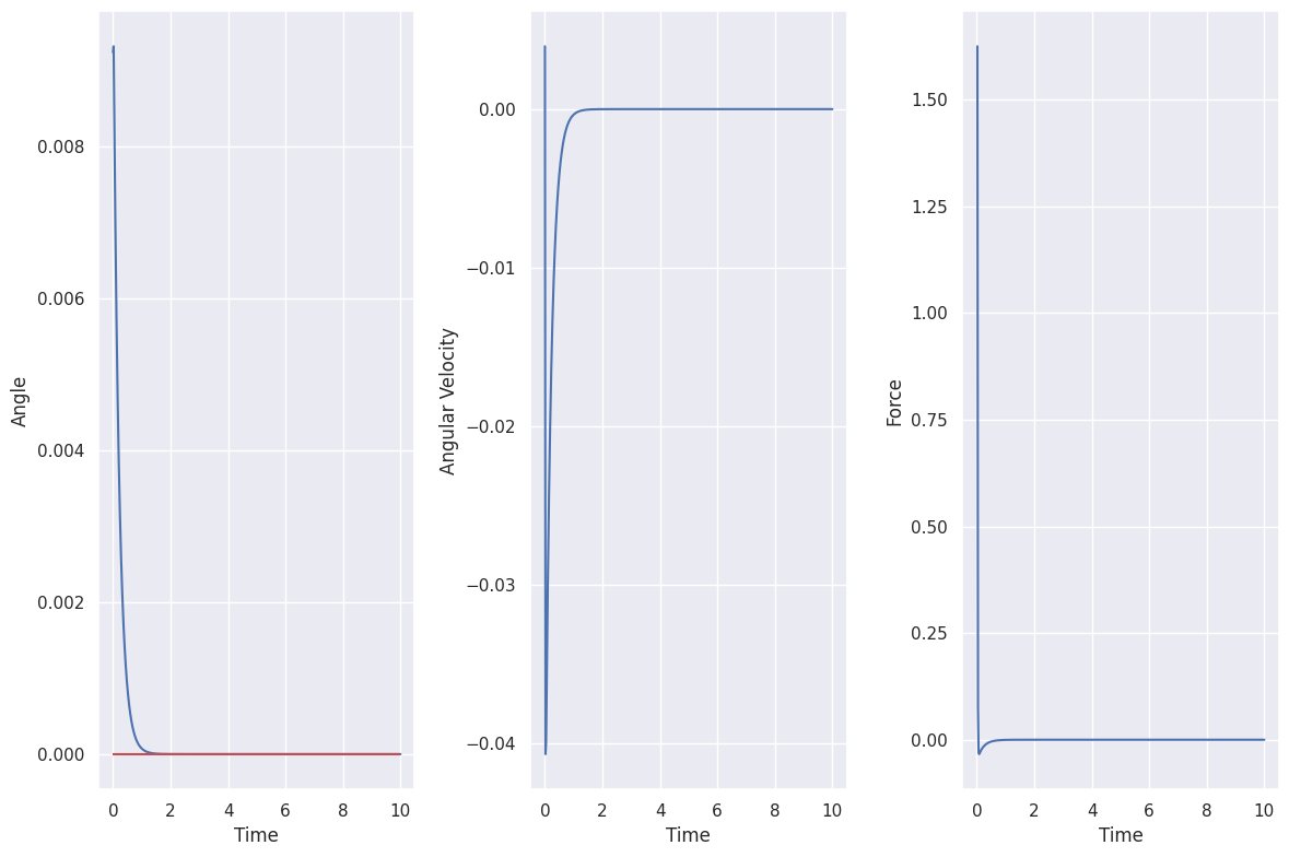
show_video(results.frames, fps=1 / env.dt, title="PID Control")

error: XDG_RUNTIME_DIR not set in the environment.

PID Control

T = np.arange(len(observations)) * env.dt
plot_inverted_pendulum_results(T, r, observations[:, [2, 3]], actions)

../_images/64cf368560e751524fb8ae19b08a26bb9ecd8d6e66cbcc7556a45360861daec7.png

Full-State Feedback#

Full-State Feedback (FSF), or pole placement, is a method employed in feedback control system theory to place the closed-loop poles of a system in pre-determined locations in the s-plane. Placing poles is desirable because the location of the poles corresponds directly to the eigenvalues of the system, which control the characteristics of the response of the system. The system must be considered controllable in order to implement this method.

We want to design a controller such that we can place the poles (eigenvalues) of our system at desired locations.

We assume that we have a single-input LTI system with the following state-space representation:

\[\begin{split} \dot{\mathbf{x}}(t) = A \mathbf{x}(t) + B \mathbf{u}(t)\\ \mathbf{y}(t) = C \mathbf{x}(t) \end{split}\]

We choose the following control law:

\[ \mathbf{u}(t) = k_r \mathbf{r}(t) - K \mathbf{x}(t) \]

Where:

\[ k_r = \frac{-1}{C(A - BK)^{-1}B}. \]

Which is exactly the inverse of the zero frequency gain of the closed loop system.

\[\begin{split} K = \begin{bmatrix} k_1 \\ k_2 \\ \vdots \\ k_n \end{bmatrix} \end{split}\]

By replacing this into the system’s state-space representation we obtain the closed-loop dynamics:

\[\begin{split} \dot{\mathbf{x}}(t) = (A - BK) \mathbf{x}(t) + k_r B \mathbf{r}(t) \\ \mathbf{y}(t) = C \mathbf{x}(t) \end{split}\]

The poles of this new system are the eigenvalues of \(A - BK\).

The location of the eigenvalues determines the behavior of the closed loop dynamics and hence where we place the eigenvalue is the main design decision to be made. As with all other feedback design problems, there are tradeoffs between the magnitude of the control inputs, the robustness of the system to perturbations and the closed loop performance of the system, including step response, disturbance attenuation and noise injection.

Choosing Poles#

The location of the poles (eigenvalues) determines the behavior of the closed loop dynamics and hence where we place the pools is the main design decision to be made.

As with all other feedback design problems, there are tradeoffs between the magnitude of the control inputs, the robustness of the system to perturbations and the closed loop performance of the system, including step response, disturbance attenuation and noise injection.

In the case of second order systems, for which the closed loop dynamics have a characteristic polynomial of the form:

\[ \lambda(s) = s^2 + 2\zeta \omega_0 s + \omega_0^2. \]

Since we can solve for the step and frequency response of such a system analytically, we can compute different performance metrics in terms of \(\zeta\) and \(\omega_0\) and determine the desired poles of the closed loop system.

Properties of the response to reference values of a second order underdamped system (\(|\zeta| < 1\)). We define \(\phi = \arccos(\zeta)\).

Property	Value	\(\zeta = 0.5\)	\(\zeta = \frac{1}{\sqrt{2}}\)	\(\zeta = 1\)
Steady-state error	\(\frac{1}{\omega_0^2}\)	\(\frac{1}{\omega_0^2}\)	\(\frac{1}{\omega_0^2}\)	\(\frac{1}{\omega_0^2}\)
Rise time \(T_r\)	\(\frac{1}{\omega_0} \exp^{\frac{\phi}{\tan(\phi)}}\)	\(\frac{1.8}{\omega_0}\)	\(\frac{2.2}{\omega_0}\)	\(\frac{2.7}{\omega_0}\)
Overshoot \(M_p\)	\(\exp^{-\pi\frac{\zeta}{\sqrt{1-\zeta^2}}}\)	\(16\%\)	\(4\%\)	\(0\%\)
Settling time (\(\%2\)) \(T_s\)	\(\frac{4}{\zeta\omega_0}\)	\(\frac{8}{\omega_0}\)	\(\frac{5.7}{\omega_0}\)	\(\frac{7}{\omega_0}\)

../_images/20_second_order_system_poles.svg — Fig. 12 Representative step and frequency responses for second order systems. Step responses are shown in the upper half of the plot, with the location of the origin of the step response indicating the value of the eigenvalues. Frequency responses are shown in the lower half of the plot.#

Exercise 10 (Full-State Feedback Controller)

Design a Full-State Feedback controller for the Inverted Pendulum system.

Tip

Hint Use the training_classical_control.control.FullStateFeedbackController() class.

Solution to ( 10

K = ct.place(inverted_pendulum.A, inverted_pendulum.B, np.array([-30, -5]))
kr = -1 / (
    inverted_pendulum.C
    @ np.linalg.inv(inverted_pendulum.A - inverted_pendulum.B @ K)
    @ inverted_pendulum.B
)
kr = kr.item()
print(f"{K=}, {kr=}")

K=array([[-160.791,  -35.   ]]), kr=-149.99999999999997

A_fsfbk = inverted_pendulum.A - inverted_pendulum.B @ K
B_fsfbk = kr * inverted_pendulum.B
C_fsfbk = inverted_pendulum.C
D_fsfbk = inverted_pendulum.D
closed_loop = ct.ss(A_fsfbk, B_fsfbk, C_fsfbk, D_fsfbk)
print(closed_loop)

<StateSpace>: sys[8]
Inputs (1): ['u[0]']
Outputs (1): ['y[0]']
States (2): ['x[0]', 'x[1]']

A = [[   0.    1.]
     [-150.  -35.]]

B = [[ -0.]
     [150.]]

C = [[1. 0.]]

D = [[0.]]

Simulation

env = create_inverted_pendulum_environment()
n_steps = 100
T = np.arange(0, n_steps) * env.dt
x0 = np.zeros(closed_loop.nstates)
# Change slightly the initial angle
x0[0] = 0.1
# reference
r = 0.0
response = ct.input_output_response(closed_loop, T, r, x0)
actions = kr * r - K.squeeze() @ response.states
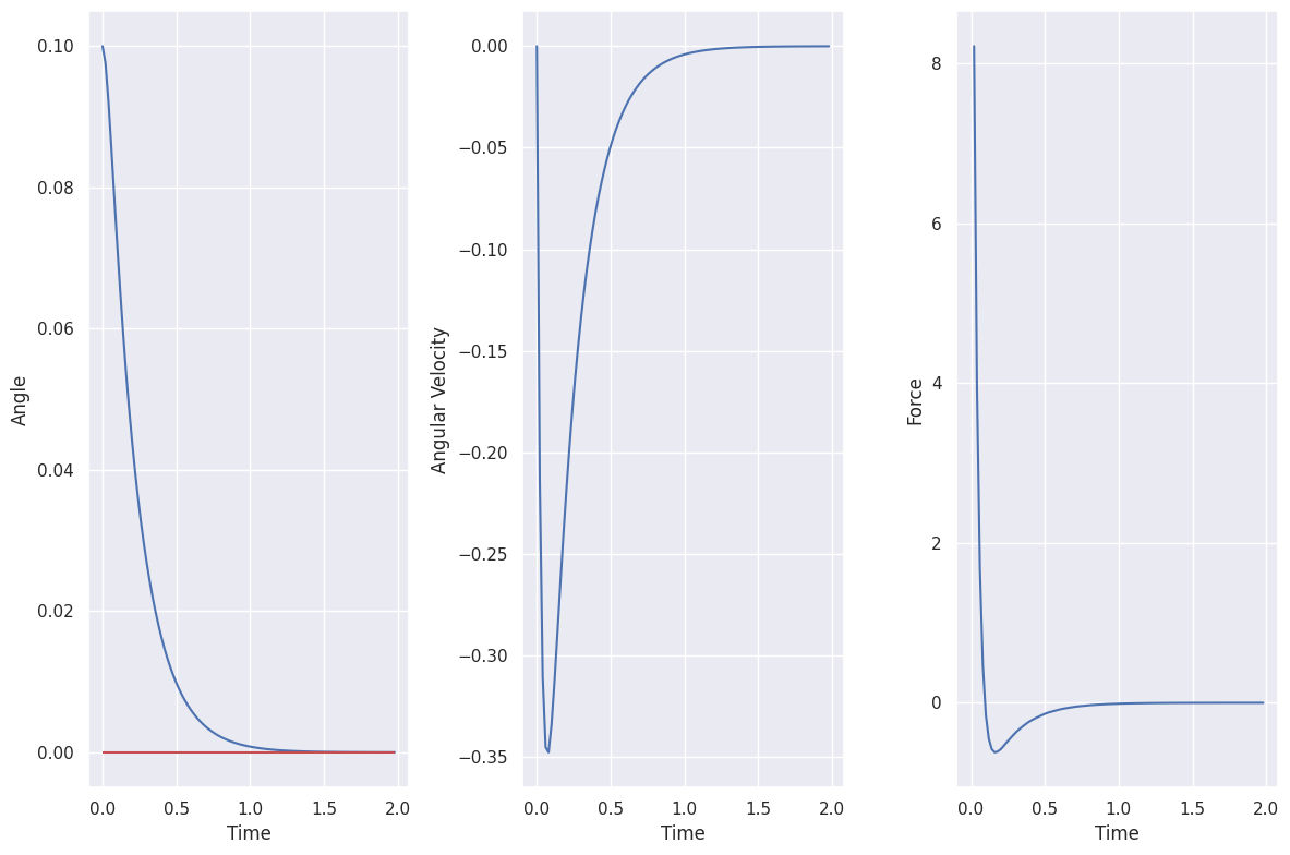
plot_inverted_pendulum_results(T, r, response.states.transpose(), actions[1:])

../_images/8c3045389f1b1fb7f64c487b9ac5c2c1ecd98737338b8824cfb2d8bf69d56ac3.png

Evaluation

max_steps = 500
env = create_inverted_pendulum_environment(max_steps=max_steps)
controller = FullStateFeedbackController(K=K, kr=kr, reference=0.0)
results = simulate_environment(env, max_steps=max_steps, controller=controller)
observations = results.observations
actions = results.actions
show_video(results.frames, fps=1 / env.dt, title="State Feedback Control")

error: XDG_RUNTIME_DIR not set in the environment.

State Feedback Control

T = np.arange(len(observations)) * env.dt
plot_inverted_pendulum_results(T, r, observations[:, [2, 3]], actions)

../_images/f95a8d857fa486d7e1811d0531e52f831507c85499a40d2db9024577526ff251.png