Introduction#
Control theory is a field of control engineering and applied mathematics that deals with influencing the behavior of dynamical systems. The objective is to drive a system towards a desired state by calculating and applying system inputs, while minimizing errors and taking into considerations any additional constraints (e.g. overshoot), and ensuring stability. The aim is often to achieve a degree of optimal and robust control performance in the presence of uncertainty.
The fundamental challenge in control theory is to determine a technically feasible way to act on a system so its behavior closely matches some desired behavior, despite uncertainties in the system’s model and external disturbances. The key elements of this control problem are:
Desired behavior The target behavior must be clearly defined as part of the control design problem. Common examples include tracking a reference trajectory, regulating around a setpoint, or optimizing some performance index.
Feasibility The control solution must satisfy constraints on the available inputs, actuator capabilities, safety limits, etc. The controller must be realizable with available technology.
Uncertainty Precise knowledge of the system is rarely possible. There will always be some uncertainty in the model parameters, unmodeled dynamics, disturbances, and measurements.
Action Control action is applied through manipulated inputs that command the system actuators. The choice of manipulated inputs and pairing with actuators is a key design decision.
Disturbances Real systems experience unknown external disturbances that affect the system behavior and must be accounted for. Rejecting disturbances is often a key control objective.
Approximate behavior Due to uncertainty, no controller can achieve perfect setpoint tracking or disturbance rejection. There will always be some approximation error. Controllers must be designed to achieve some acceptable level of performance in spite of these challenges.
Measurements Measuring the system outputs is essential for closing the feedback loop and allowing the controller to determine the effect of its inputs on the system behavior. Noise on measurements must also be accounted for.
In this training, we will focus on optimal control methods applied to linear and non-linear systems. Through the use of practical examples with a cart (double-integrator) system and an inverted pendulum system, you’ll learn how to design controllers that achieve optimal performance.
This training is structured as follows:
Introduction to Control Theory, planning and optimal control.
Dynamic Programming.
Linear Quadratic Regulator (LQR).
Model Predictive Control (MPC).
Monte-Carlo Tree Search (MCTS).
Machine Learning in Control.
Safe Learning Control.
Branches of Control Theory#
There are different branches of Control Theory:
Classical Control
deals with the behavior of linear dynamical systems with inputs, and how their behavior is modified by feedback, using the Laplace transform as a basic tool to model such systems. It is limited to single-input and single-output (SISO) system design.
The most common controllers designed using classical control theory are PID controllers.
Modern Control
deals with the behavior of linear or non-linear dynamical systems with inputs, and how their behavior is modified by feedback, using the state-space representation as a basic tool to model such systems. It can deal with multiple-input and multiple-output (MIMO) systems.
Optimal Control
deals with finding a control for a dynamical system over a period of time such that an objective function is optimized.
Adaptive Control
adapt to a controlled system with parameters which vary, or are initially uncertain.
Robust Control
an approach to controller design that explicitly deals with uncertainty.
Control Systems Classification#
There are two types of control loops:
Open-loop control (feedforward)
An open-loop control system operates without feedback, which means that the output is not measured or compared to the desired input. They are simple and inexpensive to implement. They are often used in systems where the output does not need to be precisely controlled. For example, a washing machine may use an open-loop control system to regulate the water level.
Closed-loop control (feedback)
A closed-loop control system, on the other hand, operates with feedback, meaning that the output is measured, and corrective action is taken to ensure it always matches the desired input. They are more complex and expensive to implement. However, they offer greater precision and accuracy in controlling the system’s output. Closed-loop control systems are often used in critical applications, such as aerospace engineering or medical devices
Types of Systems#
Time-Invariant (TI) or Time-Variant (TV).
Linear or Non-Linear.
Continuous-time or Discrete-time.
Deterministic or Stochastic.
Controller Design#
Problem Formulation
Modeling
Define a mathematical model that represents the system.
Determine properties of this system: Identifiability, Stability, Observability and Controllability.
Determine model’s parameters, if they’re not known already.
(Optional) Linearize model around operating point.
(Optional) If it’s a continuous-time system and we’re using a digital controller, discretize it to obtain a discrete-time system.
Control Design
Design a controller to stabilize the system.
Evaluation
Simulate the closed-loop system in order to validate the controller design.
Use controller with actual system.
Control Theory and Machine Learning#
Modern machine learning and control theory share deep theoretical connections. Framing machine learning problems as dynamical systems, which we refer to as control theory for machine learning, opens up new ways to analyze neural network training and design adaptive controllers.
Conversely, we can use machine learning to help solve large and complex control problems, which we refer to as machine learning for control theory.
Control Theory for Machine Learning#
Control theory provides key concepts to guide the development of machine learning algorithms.
Viewing neural networks like deep residual networks (ResNet) as dynamical systems allows control stability and optimality principles to ensure robust training.
Using state-space models (SSMs) in neural networks for long-range sequence modelling. Structure state-space sequence (S4) model or the more recent Mamba are examples of this.
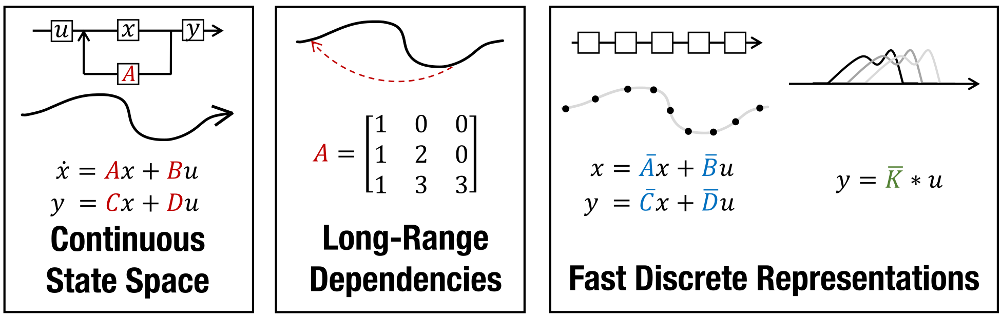
Fig. 1 Sequence modeling using state-space models (SSMs) [GGR22].#
Framing learning as an optimization problem enables control techniques like differential dynamic programming to improve convergence of algorithms like stochastic gradient descent.
The need to balance exploration and exploitation in reinforcement learning is addressed by stochastic optimal control theory.
Overall, control theory provides a rigorous mathematical framework to guarantee crucial learning properties. The system dynamics perspective further allows the training process itself to be controlled for faster convergence. Bridging machine learning with concepts from control is leading to new theories and training methods with stability and optimality guarantees.
Machine Learning for Control Theory#
Modern machine learning provides useful tools and perspectives for control theory. Framing control problems as data modeling tasks enables powerful function approximation, estimation, and optimization techniques from machine learning to be applied. For example:
Gaussian process based model learning can be used to improve the predictions of a system’s nominal model with data.
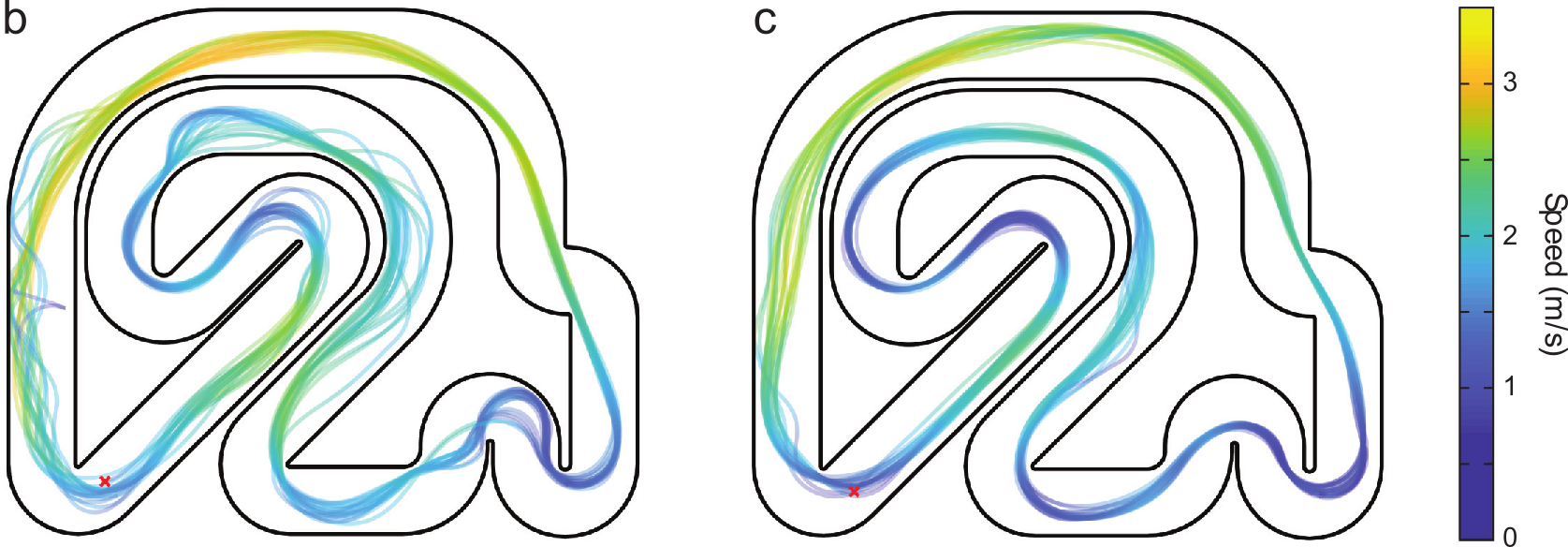
Fig. 2 Gaussian process–based MPC for autonomous racing. (b,c) The resulting trajectories of a similar approach applied to miniature radio-controlled cars, with the initial nominal controller shown in panel b and the improved trajectories after learning shown in panel c [HWMZ20].#
Neural networks can learn to approximate complex dynamics for model-predictive control (MPC).
Reinforcement learning explores optimal policies like dynamic programming to control complex robots.
Kernel methods enable non-parametric system identification without relying on predefined model structures.
The Koopman operator is a data-driven tool to infer properties and facilitate control of unknown nonlinear systems.
%%html
<iframe width="800" height="480" src="https://www.youtube.com/embed/-cdXw1MyTUA?si=S3DXY90f8QEPFddI" title="YouTube video player" frameborder="0" allow="accelerometer; autoplay; clipboard-write; encrypted-media; gyroscope; picture-in-picture; web-share" allowfullscreen></iframe>
Beyond specific techniques, a machine learning viewpoint focuses on what can be learned from data about a control system’s unknown dynamics. This data-driven approach is key for adaptive and nonlinear control of complex systems.
Control Theory and Reinforcement Learning#
The predominant sub-field of machine learning is supervised learning. Its goal is make the output of the model mimic the labels \(y\) given in the training set. In that setting, the labels give an unambiguous right answer for each of the inputs.
In reinforcement learning (RL), we do not have labels for the inputs and instead have to rely on a reward function, which indicates to the learning agent (i.e. model) when it is doing well, and when it is doing poorly.
RL studies how to use past data (experience) to enhance (learning) the future manipulation of a system, which is precisely the scope of Control Theory. Despite that, the two communities have remained disjointed and that has led to the co-development of vastly different approaches to the same problems.
The main differences between the two lie in how the system is modeled and the approaches taken to design controllers/agents:
In control theory:
we explicitly model the system using knowledge about the equations governing its behaviour, by estimating the parameters of such equations or by fitting a model on measurements from the system.
we generally deal with dynamical systems governed by differential equations.
we synthesize a controller by minimizing a cost function, in the case of optimal control.
we may have to reconstruct the state from measurements using an observer.
Whereas in reinforcement learning:
we do have to model the system and instead can directly learn the agent that maximizes the expected reward while interacting with the environment.
We generally deal with systems modelled by Markov Decision Processes (MDPs).
we train an agent by maximing a reward function.
we directly use the measurements from the environment.

Fig. 3 Feedback Control in Control Engineering#

Fig. 4 Feedback Control in Reinforcement Learning#
The two are not mutually exclusive. For example, enforcing safety constraints when using reinforcement learning can be achieved by combining it with model-predictive control (MPC).

Fig. 5 Based on the current state \(x\), a learning-based controller provides an input \(u_L = \pi_L(x) \in \mathbb{R}^m\), which is processed by the safety filter \(u = \pi_S(x, u_S)\) and applied to the real system [HWMZ20].#
Terminology#
Here are a list of terms commonly used in Reinforcement Learning, and their control counterparts:
Environment = System.
Agent (Policy) = Controller or Regulator.
Action \(a\) = Decision or Control \(u\).
Observation = Measurement.
Reward \(r\) = (Opposite of) Cost \(c\).
If you want to learn about reinforcement learning, consider attending our Safe and efficient deep reinforcement learning training.
Planning#
Planning refers to the explicit deliberation process that chooses and organizes actions by anticipating their outcomes with the goal to achieve some pre-stated objectives.
Automated planning and scheduling, sometimes denoted as simply AI planning, is a branch of artificial intelligence that concerns the realization of strategies or action sequences, typically for execution by intelligent agents, autonomous robots and unmanned vehicles. Unlike classical control problems, the solutions are complex and must be discovered and optimized in multidimensional space.
In planning we use a model of the environment/system to predict the effect of taking a certain action in a certain state. Thus it is a model-based approach.
State-Transition Systems#
A state-transition system is a 3-tuple \(\Sigma = (S, U,\gamma)\), where:
\(S = \{s_1,s_2,\dots\}\) is a finite or recursively enumerable set of states.
\(U = \{u_1,u_2,\dots\}\) is a finite or recursively enumerable set of actions.
\(\gamma: S\times U \rightarrow 2^S\) is a state transition function.
if \(u \in U\) and \(\gamma(s,u) \neq \emptyset\) then \(a\) is applicable in \(s\).
applying \(u\) in \(s\) will take the system to \(s^{\prime} \in \gamma(s,u).\)
A state-transition system can be represented by a directed labelled graph \(G = (N_G,E_G)\) where:
the nodes correspond to the states in \(S\), i.e. \(N_G = S.\)
there is an arc from \(s \in N_G\) to \(s^\prime \in N_G\), i.e.\(s \rightarrow s^\prime \in E_G\), with label \(u \in U\) if and only if \(s^\prime \in \gamma(s,u).\)
Plans#
a plan \(\pi\) is a finite sequence of actions, \(\pi = \{u_1, \dots, u_n\}\)
a planning problem is a triple \(P = (\Sigma, s_0, S_g)\), where \(\Sigma\) is a state-transition system, \(s_0 \in S\) is an initial state, and \(S_g \subset S\) is a set of goal states.
each node is written as a pair \(v = (\pi, s)\) where \(\pi\) is a plan and \(s = \gamma(s_0, \pi)\)
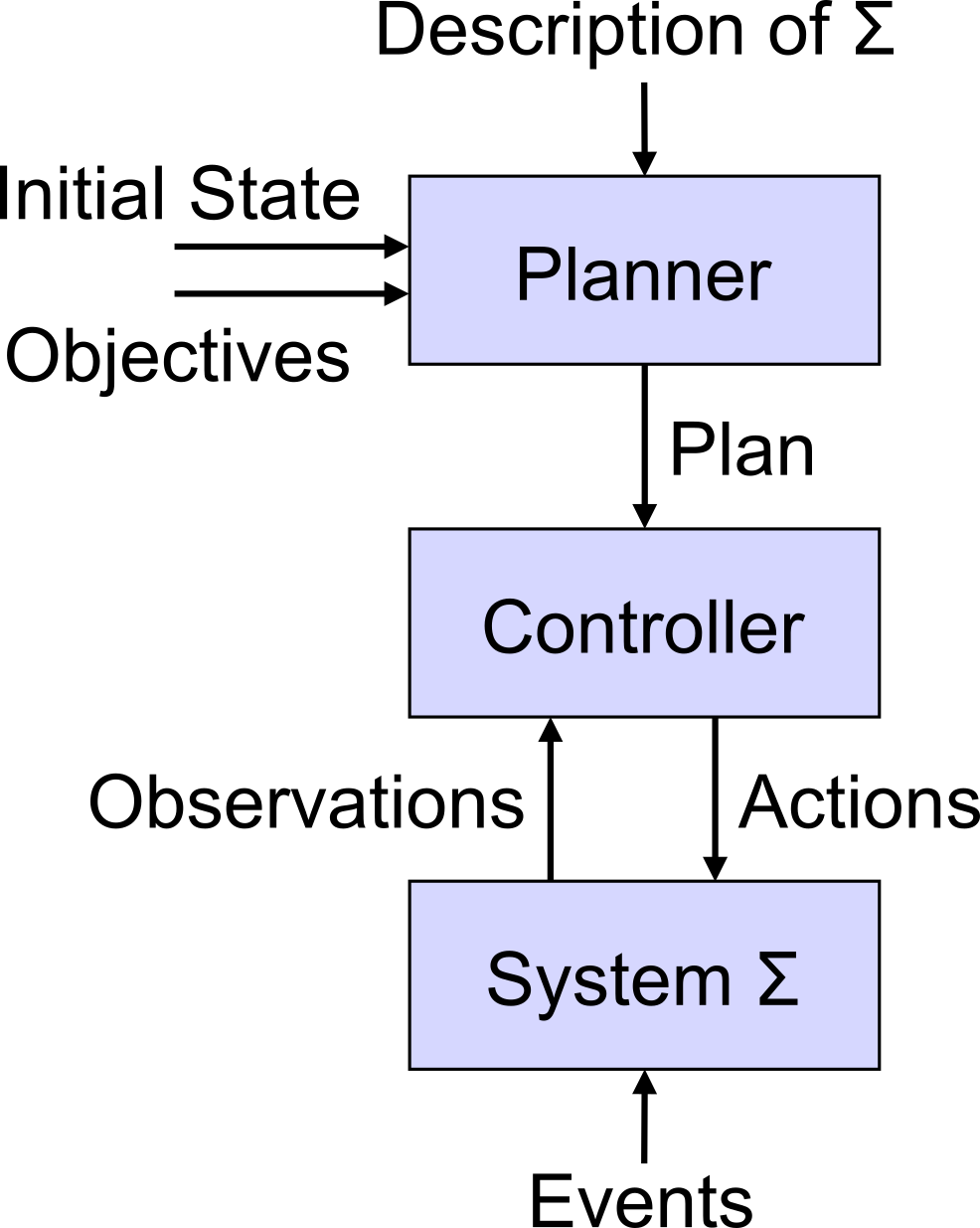
Planner:
given: description of an environment/system \(\Sigma\), initial state, and objective.
generate: plan that achieves objective.
Controller:
given: plan, current state (observation function: \(\eta:S \rightarrow O\))
generate: action.
Environment/System:
evolves as actions are executed and events occur
Optimal Control#
Optimal control theory is a branch of control theory that emerged an independent field emerged in the 1950s. It deals with finding a control for a dynamical system over a period of time such that an objective function is optimized. The fundamental idea in optimal control is to formulate the goal of control as the long-term optimization of a scalar cost function as opposed to formulating the objective as direct constraints on the system’s behaviour (e.g. overshoot) as done in classical control.
Optimal control is one of the most useful systematic methods for controller design. It has several advantages:
It gives a systematic approach to the solution of control problems.
There are normally many possible solutions to a control problem. Some are good, others are poor. Optimal control reduces this redundancy by selecting a controller that is optimal according to some cost function.
The optimal control problem is to find a control \(u^* \in \mathbf{U}\) which causes the system \(\dot{x}(t) = f(x(t), u(t))\) to follow a trajectory \(x^* \in \mathbf{X}\) that minimizes the cost (performance measure).
Continuous-time#
Discrete-time#
Variants#
There are many variants of the optimal control problem:
Finite Horizon:
\[ J(x_0, u, N) = c_N(x_N) + \sum \limits_{k = 0}^{N-1} c_k(x_k, u_k) \]Infinite Horizon:
\[ J(x_0, u) = \sum \limits_{k = 0}^{\infty} c_k(x_k, u_k) \]Stochastic finite horizon:
\[ J(x_0, u) = E\left[\sum \limits_{k=0}^{T} c_k(x_k, u_k)\right] \]
This approach is powerful for a number of reasons. First and foremost, it is very general - allowing us to specify the goal of control equally well for fully- or under-actuated, linear or nonlinear, deterministic or stochastic, and continuous or discrete systems. Second, it permits concise descriptions of potentially very complex desired behaviours, specifying the goal of control as a scalar objective (plus a list of constraints).

Fig. 6 Classification of different methods to solve optimal control problems and related formulations and solution algorithms []#
Optimal control problems solving methods can be classified in three main families: Dynamic Programming (DP), Indirect Methods based on calculus of variation and Direct Methods.
DP is helpful where the number of states is limited and the dynamics are known. It divides an optimal control problem into smaller subproblems and recursively solves each one of them.
Indirect methods rely on Pontryagin’s Minimum Principle (PMP) to derive the necessary conditions for optimality. This method uses the Hamiltonian of the system to reduce the global optimal control problem to the solution of a system of \(2N\) equations given in the form of a two-point boundary value problem (BVP).
Problems involving continuous states and control inputs benefit most from it.Direct methods rely on the discretization in time of the original optimal control problem which is then transcribed to a nonlinear programming problem (NLP) solved numerically using a well-established optimisation method.
There are many direct methods. They differ on how the variables (i.e. control and states) are discretised and on how the continuous time dynamics is approximated.
In the case of shooting and multiple shooting the control are parameterised with piecewise linear functions and the differential equations are solved via numerical integration. These approaches make use of robust and available ordinary differential equations solvers but need sensitivity analysis to compute the jacobians of the continuity and boundary conditions with respect to the initial and intermediate conditions.
In the case of state and control parameterisation (direct collocation), both states and controls are approximated with polynomial functions, therefore the continuous time differential equations are converted into algebraic constraints.
Choosing the cost function#
Choosing a cost function means translating the system’s desired physical state into a mathematical formulation.
Examples:
Minimum-time problems: \(J = t_f - t_0\)
Terminal control problems: \(J = || x(t_f) - r(t_f) ||^2\)
Minimum control-effort problems: \(J = \sum \limits_{k = t_0}^{t_f} |u(t_k)|\)
Exercise 1 (RC-Circuit Exercise)
Given the following RC circuit with an external voltage source:

Fig. 7 Schematic created using CircuitLab#
The differential equation governing the charge of capacitor is given by:
with \(y(0) = 0\) i.e. the capacitor is uncharged at \(t=0\)
The current in the circuit is given by: \(i(t) = \frac{d y(t)}{dt}\)
Questions:
Suppose our only goal is to charge the capacitor as quickly as possible without worrying about anything else. What would be your choice for a cost function?
Suppose that we additionally want to limit the current running throught the circuit. What would then be your choice for a cost function?
Tip
State-space representation of circuit (For the curious ones)
If we wanted to represent the system in a state-space form, we could define the following state vector:
Taking the derivate of the state vector gives us:
Which is a linear system with the following matrices:
Solution to ( 1
\(c = - y(t)\)
\(c = - y(t) + \lambda i(t), \quad \lambda > 0\)