Linear Quadratic Regulator

While solving the optimal control problem (OCP) is very hard in general, there are a few very important special cases where the solutions are very accessible. Most of these involve variants on the case of linear dynamics and quadratic cost. The simplest case, called the linear quadratic regulator (LQR), is formulated as stabilizing a time-invariant linear system to the origin can be solved analytically.

For a discrete-time linear time-invariant system (LTI) described by:

\[ \mathbf{x}_{t+1} = A \mathbf{x}_t + B \mathbf{u}_t \]

where \(\mathbf{x} \in \mathbb {R} ^{n}\) (that is, \(\mathbf{x}\) is an \(n\)-dimensional real-valued vector) is the state of the system and \(\mathbf{u} \in \mathbb {R} ^{m}\) is the control input.

Finite Horizon

Given a quadratic cost function for the system in the finite-horizon case, defined as: | $\( J(\mathbf{x}_0, \mathbf{u}, N) = \mathbf{x}_N^{T} Q_N \mathbf{x}_N + \sum \limits _{k = 0}^{N-1} \mathbf{x}_k^{T}Q \mathbf{x}_k + \mathbf{u}_k^{T} R \mathbf{u}_k \)$

With \(Q_N = Q_N^T \succeq 0\), \(Q = Q^T \succeq 0\), \(R = R^T \succeq 0\).

It can be shown that the control law that minizes the cost is given by:

\[ \mathbf{u}_k = K_k \mathbf{x}_k \]

\[ \mathbf{u}_k = K_k (\mathbf{x}_T - \mathbf{x}_k) \]

With: \(K_k = -(R + B^T P_k B)^{-1} B^T P_k B\)

and \(P_k\) is found by solving the discrete time dynamic Riccati equation:

\[ P_{k-1} = Q + A^{T}P_k A - (A^{T} P_k B)(R+B^{T}P_k B)^{-1}(B^{T}P_k A) \]

With \(P_N = Q_N\)

Infinite Horizon

Given a quadratic cost function for the system in the infinite-horizon case, defined as:

\[ J(\mathbf{x}_0, \mathbf{u}) = \sum \limits _{k = 0}^{\infty} \mathbf{x}_k^{T}Q \mathbf{x}_k + \mathbf{u}_k^{T} R \mathbf{u}_k \]

With \(Q = Q^T \succeq 0\), \(R = R^T \succeq 0\).

It can be shown that the control law that minizes the cost is given by:

\[ \mathbf{u}_k = K \mathbf{x}_k \]

With: \(K = -(R + B^T P B)^{-1} B^T P B\)

and \(P\) is found by solving the discrete time algebraic Riccati equation (DARE):

\[ P = Q + A^{T}PA-(A^{T}PB)(R+B^{T}PB)^{-1}(B^{T}PA) \]

Fig. 12 LQR Block Diagram.

We can create an LQR controller using the following function:

?? build_lqr_controller

Cart

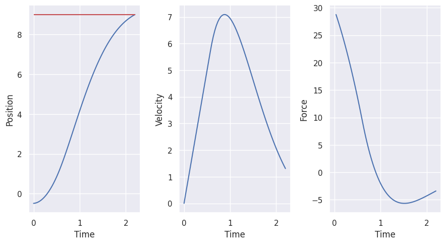
Now, we design Linear Quadratic Regulator for the Cart system.

cart_env = create_cart_environment(goal_position=9)
cart_model = build_cart_model(cart_env)
cart_simulator = Simulator(cart_model)
cart_simulator.set_param(t_step=cart_env.dt)
cart_simulator.setup()

First, we create define the cost matrices and the setpoint.

Show code cell source Hide code cell source

Q = np.diag([100, 1])
R = np.diag([10])
setpoint = np.array([cart_env.goal_position, 0.0]).reshape(-1, 1)
display_array("Q", Q)
display_array("R", R)
display_array("Setpoint", setpoint)

\[\begin{split}\displaystyle \begin{equation*}Q = \begin{bmatrix}100 &0 \\0 &1 \\\end{bmatrix}\end{equation*}\end{split}\]

\[\begin{split}\displaystyle \begin{equation*}R = \begin{bmatrix}10 \\\end{bmatrix}\end{equation*}\end{split}\]

\[\begin{split}\displaystyle \begin{equation*}Setpoint = \begin{bmatrix}9.0 \\0.0 \\\end{bmatrix}\end{equation*}\end{split}\]

We then create an instance of LQR from the do_mpc package using the already defined build_lqr_controller function.

cart_lqr_controller = build_lqr_controller(
    model=cart_model,
    t_step=cart_env.dt,
    n_horizon=None,
    setpoint=setpoint,
    Q=Q,
    R=R,
)

SImulation

Now, we simulate the closed-loop system for 50 steps:

Show code cell source Hide code cell source

cart_lqr_controller.reset_history()
cart_simulator.reset_history()
x0 = np.zeros((2, 1))
cart_simulator.x0 = x0
for _ in range(200):
    u = cart_lqr_controller.make_step(x0)
    x0 = cart_simulator.make_step(u)

animate_cart_simulation(cart_lqr_controller.data, reference=cart_env.goal_position)

Evaluation

Finally, we evaluate the controller on the actual environment.

class LQRController:
    def __init__(self, K: NDArray, setpoint: NDArray) -> None:
        self.K = K
        self.setpoint = setpoint.reshape(-1)

    def act(self, observation: NDArray) -> NDArray:
        action = self.K @ (observation - self.setpoint)
        return action

Show code cell source Hide code cell source

cart_controller = LQRController(K=cart_lqr_controller.K, setpoint=setpoint)
results = simulate_environment(cart_env, max_steps=200, controller=cart_controller)
show_video(results.frames, fps=1 / cart_env.dt)

error: XDG_RUNTIME_DIR not set in the environment.

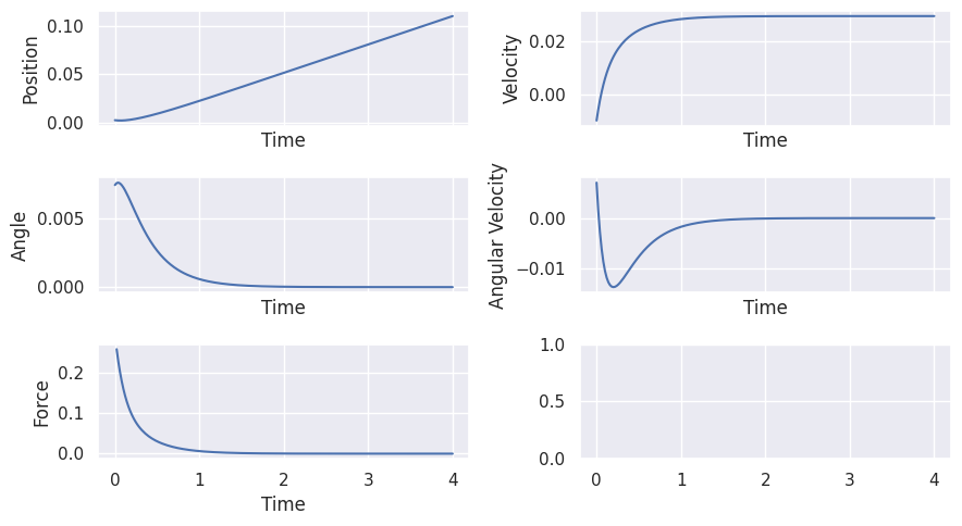
Inverted Pendulum

Exercise

Exercise 3 (Inverted Pendulum LQR Controller)

Design an LQR controller to keep the inverted pendulum upright by following these steps:

1. Define the \(Q\) and \(R\) matrices.

2. Define setpoint \(\begin{bmatrix}\theta_s \\ \dot{\theta}_s\end{bmatrix} = \begin{bmatrix}0.0 \\ 0.0 \end{bmatrix}\).

3. Create an lqr controller by calling the build_lqr_controller function and passing the appropriate arguments.

4. Simulate the system using the simulator and the controller.

5. Evaluate the controller on the environment.

Solution to ( 3

We first need the environment, linear model and simulator:

inverted_pendulum_env = create_inverted_pendulum_environment(max_steps=200)
inverted_pendulum_model = build_inverted_pendulum_linear_model(inverted_pendulum_env)
inverted_pendulum_simulator = Simulator(inverted_pendulum_model)
inverted_pendulum_simulator.set_param(t_step=inverted_pendulum_env.dt)
inverted_pendulum_simulator.setup()

The goal is to keep the inverted pendulum upright. For that we define the following objective matrices and setpoint:

Show code cell source Hide code cell source

Q = np.diag([100, 1])
R = np.diag([10])
setpoint = np.zeros((2, 1))
display_array("Q", Q)
display_array("R", R)
display_array("Setpoint", setpoint)

\[\begin{split}\displaystyle \begin{equation*}Q = \begin{bmatrix}100 &0 \\0 &1 \\\end{bmatrix}\end{equation*}\end{split}\]

\[\begin{split}\displaystyle \begin{equation*}R = \begin{bmatrix}10 \\\end{bmatrix}\end{equation*}\end{split}\]

\[\begin{split}\displaystyle \begin{equation*}Setpoint = \begin{bmatrix}0.0 \\0.0 \\\end{bmatrix}\end{equation*}\end{split}\]

We then create the controller:

inverted_pendulum_lqr_controller = build_lqr_controller(
    model=inverted_pendulum_model,
    t_step=inverted_pendulum_env.dt,
    n_horizon=None,
    setpoint=setpoint,
    Q=Q,
    R=R,
)

Simulation

Show code cell source Hide code cell source

inverted_pendulum_lqr_controller.reset_history()
inverted_pendulum_simulator.reset_history()
x0 = np.zeros((2, 1))
x0[0] = 0.01
inverted_pendulum_simulator.x0 = x0

for k in range(50):
    u0 = inverted_pendulum_lqr_controller.make_step(x0)
    x0 = inverted_pendulum_simulator.make_step(u0)

animate_inverted_pendulum_simulation(inverted_pendulum_lqr_controller.data)

Evaluation

class LQRController:
    def __init__(self, K: NDArray) -> None:
        self.K = K

    def act(self, observation: NDArray) -> NDArray:
        return self.K @ observation[[2, 3]]

Show code cell source Hide code cell source

lqr_controller = LQRController(inverted_pendulum_lqr_controller.K)
results = simulate_environment(
    inverted_pendulum_env, max_steps=200, controller=lqr_controller
)
show_video(results.frames, fps=1 / inverted_pendulum_env.dt)

error: XDG_RUNTIME_DIR not set in the environment.

Iterative Linear Quadratic Regulator

Iterative Linear Quadratic Regulator (iLQR) is an extension of LQR control to non-linear system with non-linear quadratic costs.

The idea is to approximate the cost and dynamics as quadratic and affine, respectively, then exactly solve the resulting LQR problem.

The basic flow of the algorithm is:

1. Initialize with initial state \(\mathbf{x}_0\) and initial control sequence \(\mathbf{U} = \{\mathbf{u}_{0}, \mathbf{u}_{1}, \dots, \mathbf{u}_{N-1}\}\).

2. Do a forward pass using the non-linear dynamics, i.e. simulate the system using \((\mathbf{x}_0, \mathbf{U})\) to get the trajectory through state space, \(\mathbf{X}\), that results from applying the control sequence \(\mathbf{X}\) starting in \(\mathbf{x}_0\).

3. Do a backward pass, estimate the value function and dynamics for each \((\mathbf{x}, \mathbf{u})\) in the state-space and control signal trajectories.

4. Calculate an updated control signal \(\hat{\mathbf{U}}\) and evaluate cost of trajectory resulting from \((\mathbf{x}_0, \hat{\mathbf{U}})\).

   1. If \(|(\textrm{cost}(x_0, \hat{\textbf{U}}) - \textrm{cost}(x_0, \textbf{U})| < \textrm{threshold},\) then we’ve converged and exit.

   2. If \(\textrm{cost}(x_0, \hat{\textbf{U}}) < \textrm{cost}(x_0, \textbf{U}),\) then set \(\textbf{U} = \hat{\textbf{U}},\) and change the update size to be more aggressive. Go back to step 2.

   3. If \(\textrm{cost}(x_0, \hat{\textbf{U}}) \geq \textrm{cost}(x_0, \textbf{U}),\) change the update size to be more modest. Go back to step 3.

Note

Mathematical Derivation

Given a discrete-time non-linear system with state-space representation:

\[ \mathbf{x}_{t+1} = f(\mathbf{x}_t, \mathbf{u}_t) \]

we approximate it with a first-order Taylor-series expansion about nominal trajectories \(\mathbf{X} = \{\mathbf{x}_0, \dots, \mathbf{x}_N\}, \mathbf{U} = \{ \mathbf{u}_0, \dots, \mathbf{u}_N \}\):

\[\begin{split} \begin{array}{lll} \mathbf{x}_{t+1} + \delta\mathbf{x}_{t+1} &= f(\mathbf{x}_t + \delta \mathbf{x}_t, \mathbf{u}_t + \delta \mathbf{u}_t) \\ & \approx f(\mathbf{x}_t, \mathbf{u}_t) + \frac{\partial f}{\partial \mathbf{x}}|_{\mathbf{x}_t, \mathbf{u}_t}\delta\mathbf{x}_t + \frac{\partial f}{\partial \mathbf{u}}|_{\mathbf{x}_t, \mathbf{u}_t}\delta\mathbf{u}_t\\ \delta\mathbf{x}_{t+1} &= A_t\delta\mathbf{x}_t + B_t\delta\mathbf{u}_t \end{array} \end{split}\]

with \(A_t = A(\mathbf{x}_t, \mathbf{u}_t) = \frac{\partial f}{\partial \mathbf{x}}|_{\mathbf{x}_t, \mathbf{u}_t}\) and \(B_t = B(\mathbf{x}_t, \mathbf{u}_t) = \frac{\partial f}{\partial \mathbf{u}}|_{\mathbf{x}_t, \mathbf{u}_t}\)

Given a general cost function that is not linear-quadratic, we use a second-order Taylor Series Expansion to linearize the dynamics into a form common for optimal control problems:

\[\begin{split} \begin{array}{lll} J_N(\mathbf{x}_0, \mathbf{U}) &= l_f(\mathbf{x}_N) + \sum \limits_{t=1}^{N-1} l(\mathbf{x}_t, \mathbf{u}_t)\\ &\approx \frac{1}{2} \mathbf{x}^T_N Q \mathbf{x}_N + q_N^T \mathbf{x}_N + \sum \limits_{t=1}^{N-1} \frac{1}{2} \mathbf{x}^T_t Q_t \mathbf{x}_t + \frac{1}{2} \mathbf{u}^T_t R_t \mathbf{u}_t + \frac{1}{2} \mathbf{x}^T_t H_t \mathbf{u}_t + \frac{1}{2} \mathbf{u}^T_t H_t^T \mathbf{x}_t + q_t^T \mathbf{x}_t + + r_t^T \mathbf{u}_t \end{array} \end{split}\]

We define the following variables for convenience:

\[\begin{split} \begin{array}{lll} l_x &:= \frac{\partial l}{\partial \mathbf{x}}|_{\mathbf{x}_t, \mathbf{u}_t} = Q_t \mathbf{x}_t + q_t \\ l_u &:= \frac{\partial l}{\partial \mathbf{u}}|_{\mathbf{x}_t, \mathbf{u}_t} = R_t \mathbf{u}_t + r_t \\ l_{xx} &:= \frac{\partial^2 l}{\partial \mathbf{x}^2}|_{\mathbf{x}_t, \mathbf{u}_t} = Q_t \\ l_{uu} &:= \frac{\partial^2 l}{\partial \mathbf{u}^2}|_{\mathbf{x}_t, \mathbf{u}_t} = R_t \\ l_{xu} &:= \frac{\partial^2 l}{\partial \mathbf{x}\mathbf{u}}|_{\mathbf{x}_t, \mathbf{u}_t} = H_t \\ l_{ux} &:= \frac{\partial^2 l}{\partial \mathbf{u}\mathbf{x}}|_{\mathbf{x}_t, \mathbf{u}_t} = H_t^T \end{array} \end{split}\]

We can apply Bellman’s Principle of Optimality to define the optimal cost-to-go:

\[\begin{split} \begin{array}{lll} V_N(\mathbf{x}_N) &= g_f(\mathbf{x}_N)\\ V_{t}(\mathbf{x}_t) &= \displaystyle \min_u {g(\mathbf{x}_{t}, \mathbf{u}_{t}) + V_{t+1}(f(\mathbf{x}_{t}, \mathbf{u}_{N-t}))}\\ V_{t}(\mathbf{x}_t) &= \displaystyle \min_u Q_{t}(\mathbf{x}_{t}, \mathbf{u}_{t}) \end{array}\\ \end{split}\]

The \(Q\)-function is the discrete-time analogue of the Hamiltonian, sometimes known as the pseudo-Hamiltonian.

We approximate the cost-to-go function as locally quadratic near the nominal trajectory gives us (we drop the time index in some of the equations for the sake of readability):

\[ \delta V(\mathbf{x}) = s^T \delta\mathbf{x} + \frac{1}{2} \delta\mathbf{x}^T S \delta\mathbf{x} \]

with \(s = \frac{\partial V}{\partial \mathbf{x}}|_{\mathbf{x}}, S = \frac{\partial^2 V}{\partial \mathbf{x}^2}|_{\mathbf{x}}\)

Similarily:

\[\begin{split} \delta Q(\mathbf{x}, \mathbf{u}) = \frac{1}{2} \begin{bmatrix} \delta\mathbf{x} \\ \delta\mathbf{u} \end{bmatrix}^T \begin{bmatrix} Q_{xx} & Q_{xu} \\ Q_{ux} & Q_{uu} \end{bmatrix} \begin{bmatrix} \delta\mathbf{x} \\ \delta\mathbf{u} \end{bmatrix} + \begin{bmatrix} Q_{x} \\ Q_{u} \end{bmatrix}^T \begin{bmatrix} \delta\mathbf{x} \\ \delta\mathbf{u} \end{bmatrix} \end{split}\]

with:

\[\begin{split} \begin{array}{lll} Q_x &= l_x + s_{t+1} A_t \\ Q_u &= l_u + s_{t+1} B_t \\ Q_{xx} &= l_{xx} + A_t^T S_{t+1} A_t \\ Q_{uu} &= l_{uu} + B_t^T S_{t+1} B_t \\ Q_{ux} &= l_{ux} + B_t^T S_{t+1} A_t \end{array} \end{split}\]

The optimal control modification \(\delta\mathbf{u}^∗\) for some state perturbation \(\delta\mathbf{x}\), is obtained by minimizing the quadratic model:

\[ \delta\mathbf{u}^∗(\delta\mathbf{x}) = \displaystyle\arg\min_{\delta\mathbf{u}} Q(\delta\mathbf{x}, \delta\mathbf{u}) = k + K\delta\mathbf{x} \]

This is a locally-linear feedback policy with:

\[\begin{split} k := -Q_{uu}^{-1}Q_u\\ K := -Q_{uu}^{-1}Q_{ux} \end{split}\]

Plugging this back into the expansion of \(Q\), a quadratic model of \(V\) is obtained. After simplification it is:

\[\begin{split} \begin{array}{lll} \Delta V &= \frac{1}{2} k^T Q_{uu} k + k^T Q_u\\ s &= Q_x + K^T Q_{uu} k + K^T Q_u + Q_{ux}^T k\\ S &= Q_{xx} + K^T Q_{uu} K + K^T Q_{ux} + Q_{ux}^T K \end{array} \end{split}\]

Once these terms are computed, a forward pass computes a new trajectory:

\[\begin{split} \begin{array}{lll} \hat{x}_0 &= x_0\\ \hat{u}_t &= u_t + k_t + K_t(\hat{x}_t - x_t)\\ \hat{x}_{t+1} &= f(\hat{x}_t, \hat{u}_t) \end{array} \end{split}\]