Systems

Cart (Double Integrator)

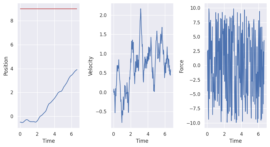
The double integrator is a canonical example of a second-order control system. It models the dynamics of a simple mass in one-dimensional space under the effect of a time-varying force input.

Show code cell source Hide code cell source

cart_env = create_cart_environment(goal_position=9)
results = simulate_environment(cart_env)
show_video(results.frames, fps=1 / cart_env.dt)

error: XDG_RUNTIME_DIR not set in the environment.

For the simulation we will use a modified version of the Mountain Car Continuous environment from gymnasium.

It has the following possible action and observations:

Num	Action	Control Min	Control Max
0	Force applied on the cart	-10	10

Num	Observation	Min	Max
0	position of the cart along the linear surface	-3.0	3.0
1	linear velocity of the cart	-Inf	Inf

Model

The differential equations which represent a one-dimensional double integrator are:

\[\begin{split} \begin{array}{ll} \ddot {q}(t) &= u(t)\\ y(t) &= q(t) \end{array} \end{split}\]

where \(\displaystyle q(t),u(t)\in \mathbb {R}\).

It is clear that the control input \(u\) is the second derivative of the output \(q\).

Defining the state-vector vector as \(X = \begin{bmatrix}x_1\\{x_2}\\\end{bmatrix} = \begin{bmatrix}q\\{\dot {q}}\\\end{bmatrix}\), gives us the following state-space representation:

\[\begin{split} \dot{X} = \begin{bmatrix}{\dot{x}_1}\\{\dot {x}_2}\\\end{bmatrix} = \begin{bmatrix}{x_2}\\{u}\\\end{bmatrix} \end{split}\]

This leads to a linear state-space model with matrices:

\[\begin{split} A = \begin{bmatrix} 0 & 1 \\ 0 & 0\\ \end{bmatrix}; B = \begin{bmatrix} 0 \\ 1 \end{bmatrix}; C = \begin{bmatrix} 1 & 0 \\ \end{bmatrix}; D = \begin{bmatrix} 0 \end{bmatrix} \end{split}\]

cart_model = build_cart_model(cart_env)

Simulator

cart_simulator = Simulator(cart_model)
cart_simulator.set_param(t_step=cart_env.dt)
cart_simulator.setup()

We then use the simulator to simulate the model starting from the same initial state as the environment and using the same inputs.

Show code cell source Hide code cell source

cart_simulator.reset_history()
x0 = results.observations[0]
cart_simulator.x0 = x0
for i in range(len(results.observations) - 1):
    u = results.actions[[i]]
    x0 = cart_simulator.make_step(u)

animate_cart_simulation(cart_simulator.data)

Inverted Pendulum

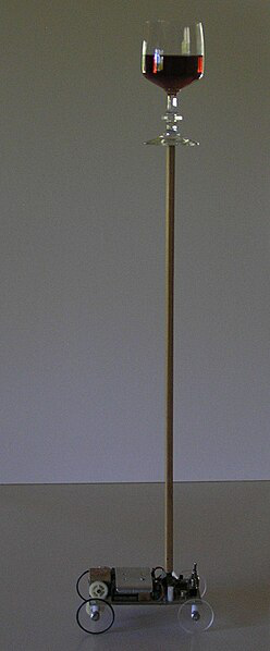
Fig. 10 Balancing cart, a simple robotics system circa 1976 - Wikipedia.

An inverted pendulum is a pendulum that has its center of mass above its pivot point. It is unstable and without additional help will fall over.

The inverted pendulum is a classic problem in dynamics and control theory and is used as a benchmark for testing control strategies. It is often implemented with the pivot point mounted on a cart that can move horizontally under control of an electronic servo system as shown in the image.

For the simulation we will use a modified version of the CartPole environment from gymnasium.

It has the following possible action and observations:

Num	Action	Control Min	Control Max
0	Force applied on the cart	-30	30

Num	Observation	Min	Max
0	position of the cart along the linear surface	-3.0	3.0
1	linear velocity of the cart	-Inf	Inf
2	vertical angle of the pole on the cart	-24	24
3	angular velocity of the pole on the cart	-Inf	Inf

error: XDG_RUNTIME_DIR not set in the environment.

Dynamic Model

Fig. 11 Inverted pendulum model diagram. Taken from this document.

• \(x\): distance along the horizontal axis from some reference point.

• \(\theta\): angle of the pendulum.

• \(m_c\): mass of the cart.

• \(m_p\): mass of the pole.

• \(l\): length of the pole.

• \(F\): force applied on the cart.

Application of Newtonian physics to this system leads to the following model[1][2]:

\[\begin{split} \ddot{x} = \frac{1}{m_p\cos^2(\theta) - \frac{4}{3}(m_c + m_p)} \left[ m_p g \sin(\theta) \cos(\theta) - \frac{4}{3}(F + m_p \frac{l}{2} \dot{\theta}^2 \sin(\theta)) \right]\\ \ddot{\theta} = \frac{1}{\frac{4}{3}(m_c + m_p)l - m_p l \cos^2(\theta)} \left[ (m_c + m_p)g\sin(\theta) - \cos(\theta) (F + m_p l \dot{\theta}^2 \sin(\theta)) \right] \end{split}\]

We can convert this to a state-space representation with input \(\mathbf{u} = F\) and state\(\mathbf{X}\):

\[\begin{split} \mathbf{X} = \begin{bmatrix} x_1 \\ x_2 \\ x_3 \\ x_4 \end{bmatrix} = \begin{bmatrix} x \\ \dot{x} \\ \theta \\ \dot{\theta} \end{bmatrix} \end{split}\]

\[\begin{split} \dot{\mathbf{X}} = \begin{bmatrix} \dot{x}_1 \\ \dot{x}_2 \\ \dot{x}_3 \\ \dot{x}_4 \end{bmatrix} = \begin{bmatrix} x_2 \\ \frac{1}{m_p\cos^2(x_3) - \frac{4}{3}(m_c + m_p)} \left[ m_p g \sin(x_3) \cos(x_3) - \frac{4}{3}(F + m_p l x_4^2 \sin(x_3)) \right]\\ \\ x_4 \\ \frac{1}{\frac{4}{3}(m_c + m_p)l - m_p l \cos^2(x_3)} \left[ (m_c + m_p)g\sin(x_3) - \cos(x_3) (\mathbf{u} + m_p l x_4^2 \sin(x_3)) \right] \\ \end{bmatrix} \end{split}\]

For simple cases (e.g. linear controller design), we’re only interested in controlling the pendulum’s angle, so we can ignore the first 2 states and redefine the state vector as.

\[\begin{split} \mathbf{X} = \begin{bmatrix} x_1 \\ x_2 \end{bmatrix} = \begin{bmatrix} \theta \\ \dot{\theta} \end{bmatrix} \end{split}\]

Which gives us:

\[\begin{split} \dot{\mathbf{X}} = \begin{bmatrix} \dot{x}_1 \\ \dot{x}_2 \end{bmatrix} = \begin{bmatrix} x_2 \\ \frac{1}{\frac{4}{3}(m_c + m_p)l - m_p l\cos^2(x_1)} \left[ (m_c + m_p)g\sin(x_1) - \cos(x_1) (\mathbf{u} + m_p l x_2^2 \sin(x_1))\right] \\ \end{bmatrix} \end{split}\]

These equations are nonlinear. However, for small departures of \(x_1\) (i.e. \(\theta\)) from the vertical position we can linearize about \(x_1 = 0\), \(x_2 = 0\). This is called the small-angle approximation.

Applying the approximation gives us:

\[\begin{split} \dot{\mathbf{X}} = \begin{bmatrix} \dot{x}_1 \\ \dot{x}_2 \end{bmatrix} = \begin{bmatrix} x_2 \\ \frac{1}{m_c l} \left[ - \mathbf{u} + (m_c + m_p) g x_1 \right] \\ \end{bmatrix} = \begin{bmatrix} 0 & 1\\ \frac{(m_c + m_p)g}{m_c l} & 0\\ \end{bmatrix} \begin{bmatrix} x_1 \\ x_2 \end{bmatrix} + \begin{bmatrix} 0 \\ -\frac{1}{m_c l} \end{bmatrix} \begin{bmatrix} \mathbf{u}\\ \end{bmatrix} \end{split}\]

This leads to a linear state-space model with matrices:

\[\begin{split} A = \begin{bmatrix} 0 & 1 \\ \frac{(m_c + m_p)g}{m_c l} & 0\\ \end{bmatrix}; B = \begin{bmatrix} 0 \\ -\frac{1}{m_c l} \end{bmatrix}; C = \begin{bmatrix} 1 & 0 \\ \end{bmatrix}; D = \begin{bmatrix} 0 \end{bmatrix} \end{split}\]

Linear Model

inverted_pendulum_linear_model = build_inverted_pendulum_linear_model(
    inverted_pendulum_env
)

Simulator

inverted_pendulum_linear_simulator = Simulator(inverted_pendulum_linear_model)
inverted_pendulum_linear_simulator.set_param(t_step=inverted_pendulum_env.dt)
inverted_pendulum_linear_simulator.setup()

We then use the simulator to simulate the the model starting from the same initial state as the environment and using the same inputs.

Show code cell source Hide code cell source

x0 = results.observations[0, 2:]

inverted_pendulum_linear_simulator.reset_history()
inverted_pendulum_linear_simulator.x0 = x0

for i in range(len(results.observations) - 1):
    u = results.actions[[i]]
    x0 = inverted_pendulum_linear_simulator.make_step(u)

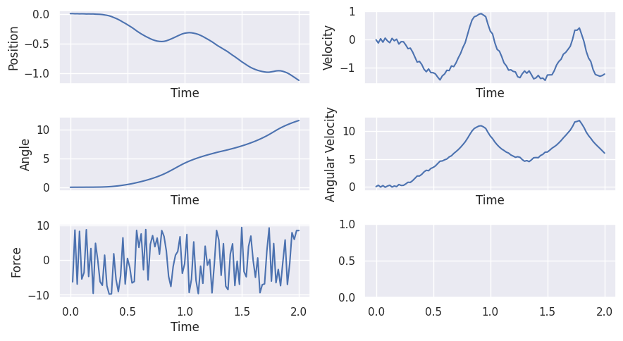
animate_inverted_pendulum_simulation(inverted_pendulum_linear_simulator.data)

We notice that the simulation quickly diverges as the states moves away from the origin. The model should still be good for the purpose of controlling the system to stay near the origin.

Full Non-Linear Model

inverted_pendulum_nonlinear_model = build_inverted_pendulum_nonlinear_model(
    inverted_pendulum_env
)

Simulator

inverted_pendulum_nonlinear_simulator = Simulator(inverted_pendulum_nonlinear_model)
params_simulator = {
    # Note: cvode doesn't support DAE systems.
    "integration_tool": "idas",
    "abstol": 1e-8,
    "reltol": 1e-8,
    "t_step": inverted_pendulum_env.dt,
}
inverted_pendulum_nonlinear_simulator.set_param(**params_simulator)
inverted_pendulum_nonlinear_simulator.setup()

We then use the simulator to simulate the the model starting from the same initial state as the environment and using the same inputs.

Show code cell source Hide code cell source

x0 = results.observations[0]

inverted_pendulum_nonlinear_simulator.reset_history()
inverted_pendulum_nonlinear_simulator.x0 = x0

for i in range(len(results.observations) - 1):
    u = results.actions[[i]]
    x0 = inverted_pendulum_nonlinear_simulator.make_step(u)

animate_full_inverted_pendulum_simulation(inverted_pendulum_nonlinear_simulator.data)

---

[1]

for the sake of simplicity we will ignore friction.

[2]

for a detailed derivation of these equations refer to this document.