Model Predictive Control#
Unfortunately, the analytically convenient linear quadratic problem formulations are often not satisfactory. There are two main reasons for this:
The system may be nonlinear, and it may be inappropriate to use for control purposes. Moreover, some of the control variables may be naturally discrete, and this is incompatible with the linear system viewpoint.
There may be control and/or state constraints, which are not handled adequately through quadratic penalty terms in the cost function. For example, the motion of a car may be constrained by the presence of obstacles and hardware limitations. The solution obtained from a linear quadratic model may not be suitable for such a problem, because quadratic penalties treat constraints “softly” and may produce trajectories that violate the constraints.
Model Predictive Control (MPC), also referred to as Receding Horizon Control and Moving Horizon Optimal Control, is a control algorithm based on solving an on-line optimal control problem. A receding horizon approach is used which can be summarized in the following steps:
At time \(t\) and for the current state \(x_t\), solve, on-line, an open-loop optimal control problem over some future interval taking account the current and future constraints.
Apply the first step in the optimal control sequence.
Repeat the procedure at time \(t + 1\) using the current state \(x_{t + 1}\).

Fig. 13 Illustration of the problem solved by MPC at state \(x_k\). We minimize the cost function over the next \(l\) stages. We then apply the control of the optimizing sequence up to the control horizon. In most cases, the control horizon is set to 1.#
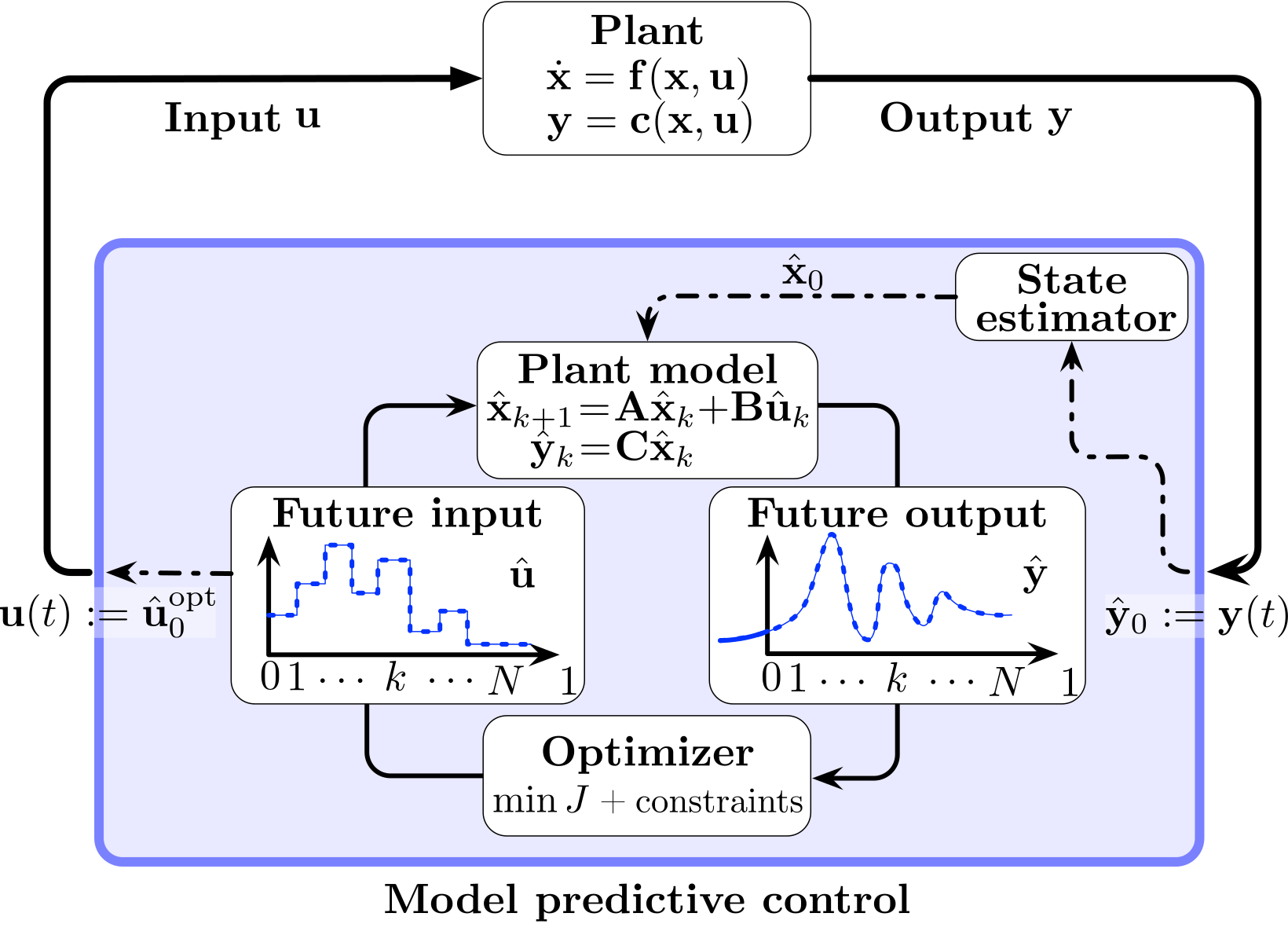
Fig. 14 MPC Block Diagram.#
A major difference between MPC and finite-state stochastic control problems that are popular in the RL/artificial intelligence literature is that in MPC the state and control spaces are continuous/infinite, such as for example in self-driving cars, the control of aircraft and drones, or the operation of chemical processes
?? build_mpc_controller
build_mpc_controller does the following:
First, it creates an instance of the MPC class is generated with the passeed model.
It configures this object with parameters such as the time step and the horizon as well as parameters that are specific to the solver we are using.
It then sets the control objective using the passed terminal and stage costs.
It also restricts the input force by adding an optional penalty.
After that, it sets upper and lower limits for the state and force.
Finally, it sets everything up and returns the controller object.
do-mpc, the package we’re using in this training, uses CasADi (an open-source tool for nonlinear optimization and algorithmic differentiation) for the modeling part and for the different cost functions. Here’s a table of useful operators:
Operator |
Description |
Equation |
|---|---|---|
Squared-sum |
\(\sum x_i^2\) |
|
\(L_2\)-norm |
\(\sqrt{\sum x_i^2}\) |
|
\(L_1\)-norm |
$\sum |
|
Quadratic Form |
\(x^T A x\) |
|
Bilinear Form |
\(x^T A y\) |
Cart#
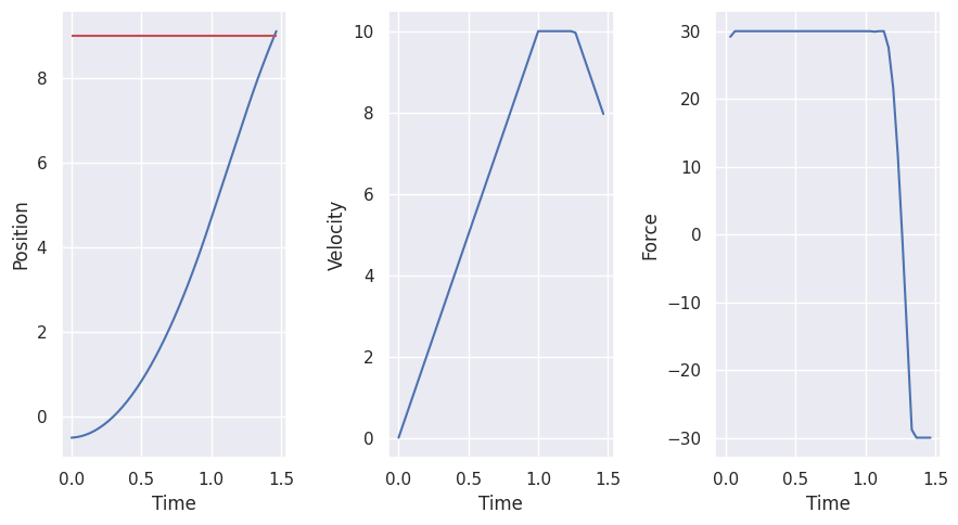
Now, we design an MPC controller for the Cart system.
cart_env = create_cart_environment(goal_position=9)
cart_model = build_cart_model(cart_env)
cart_simulator = Simulator(cart_model)
cart_simulator.set_param(t_step=cart_env.dt)
cart_simulator.setup()
Controller#
The control objective is to move the cart to a desired position (\(x_1 = 9\)).
distance_cost = casadi.norm_2(cart_model.x["position"] - cart_env.goal_position)
terminal_cost = distance_cost
stage_cost = distance_cost
print(f"Stage Cost = {stage_cost}")
print(f"Terminal Cost = {terminal_cost}")
Stage Cost = fabs((position-9))
Terminal Cost = fabs((position-9))
We also restrict the input force.
u_penalty = {"force": 1e-3}
We define as well upper and lower limits for the state and force
x_limits = {"position": np.array([-10, 10])}
u_limits = {"force": np.array([-30, 30])}
We then create an instance of MPC from the do_mpc package using the already defined build_mpc_controller function.
cart_mpc_controller = build_mpc_controller(
    model=cart_model,
    t_step=cart_env.dt,
    n_horizon=10,
    stage_cost=stage_cost,
    terminal_cost=terminal_cost,
    u_penalty=u_penalty,
    x_limits=x_limits,
    u_limits=u_limits,
)
Simulation#
We set the initial state and simulate the closed-loop for 100 steps.
Show code cell source
%%capture
cart_mpc_controller.reset_history()
cart_simulator.reset_history()

x0 = np.random.normal(loc=np.zeros((2, 1)))
cart_simulator.x0 = x0
cart_mpc_controller.x0 = x0
cart_mpc_controller.set_initial_guess()

for k in range(100):
    u = cart_mpc_controller.make_step(x0)
    x0 = cart_simulator.make_step(u)
Evaluation#
Finally, we evaluate the controller on the actual environment.
class MPCController:
    def __init__(self, mpc: MPC) -> None:
        self.mpc = mpc
        self.mpc.reset_history()
        self.mpc.x0 = np.random.normal(loc=np.zeros((2, 1)))
        self.mpc.set_initial_guess()

    def act(self, observation: NDArray) -> NDArray:
        return self.mpc.make_step(observation.reshape(-1, 1)).ravel()
Show code cell source
%%capture
controller = MPCController(cart_mpc_controller)
results = simulate_environment(cart_env, max_steps=200, controller=controller)
error: XDG_RUNTIME_DIR not set in the environment.
 |
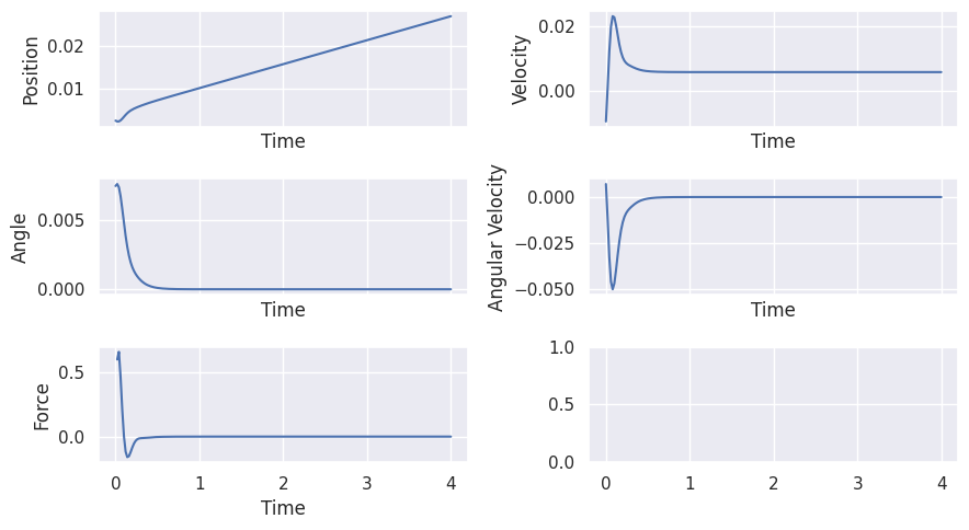
Inverted Pendulum#
Exercise (Linear)#
Exercise 4 (Linear Inverted Pendulum MPC)
Design an MPC controller for linearized inverted pendulum model to keep the pole upright by following these steps:
Define stage and terminal costs.
Define setpoint \(\begin{bmatrix}\theta_s \\ \dot{\theta}_s\end{bmatrix} = \begin{bmatrix}0.0 \\ 0.0 \end{bmatrix}\).
Define appropriate force penalty.
Create an mpc controller by calling the
build_mpc_controllerfunction and passing the appropriate arguments.Simulate the system using the simulator and the controller.
Evaluate the controller on the environment.
For each case, try different cost functions:
\(\sum \theta^2\)
\(\sum |\theta|\)
\(E_{\text{kinetic}} - E_{\text{potential}}\)
Hint
You can access the inverted pendulum’s kinetic, respectively potential, energy using inverted_pendulum_lin_model.aux["E_kinetic"], respectively inverted_pendulum_lin_model.aux["E_potential"])
Solution to ( 4
We first need the environment, linear model and simulator:
inverted_pendulum_env = create_inverted_pendulum_environment(max_steps=200)
inverted_pendulum_lin_model = build_inverted_pendulum_linear_model(
    inverted_pendulum_env
)
inverted_pendulum_lin_simulator = Simulator(inverted_pendulum_lin_model)
inverted_pendulum_lin_simulator.set_param(t_step=inverted_pendulum_env.dt)
inverted_pendulum_lin_simulator.setup()
The goal is to keep the inverted pendulum upright. For that we define the following costs, setpoint and force penalty:
setpoint = np.zeros((2, 1))
distance_cost = casadi.bilin(
    np.diag([100, 1]), inverted_pendulum_lin_model.x.cat - setpoint
)
terminal_cost = distance_cost
stage_cost = distance_cost
u_penalty = {"force": 1e-2}
display_array("Setpoint", setpoint)
print(f"{stage_cost=}")
print(f"{terminal_cost=}")
stage_cost=SX((((100*theta)*theta)+sq(dtheta)))
terminal_cost=SX((((100*theta)*theta)+sq(dtheta)))
We define as well upper and lower limits for the state and force
x_limits = {"theta": np.array([-10, 10])}
u_limits = {
    "force": np.array(
        [-inverted_pendulum_env.force_max, inverted_pendulum_env.force_max]
    )
}
After that, we create the controller:
inverted_pendulum_mpc_controller = build_mpc_controller(
    model=inverted_pendulum_lin_model,
    t_step=inverted_pendulum_env.dt,
    n_horizon=30,
    stage_cost=stage_cost,
    terminal_cost=terminal_cost,
    u_penalty=u_penalty,
    x_limits=x_limits,
    u_limits=u_limits,
)
Simulation
Show code cell source
%%capture
inverted_pendulum_mpc_controller.reset_history()
inverted_pendulum_lin_simulator.reset_history()
x0 = np.zeros((2, 1))
x0[0] = 0.01
inverted_pendulum_lin_simulator.x0 = x0

for k in range(50):
    u0 = inverted_pendulum_mpc_controller.make_step(x0)
    x0 = inverted_pendulum_lin_simulator.make_step(u0)
Evaluation
class MPCController:
    def __init__(self, mpc: do_mpc.controller.MPC) -> None:
        self.mpc = mpc
        self.mpc.reset_history()
        self.mpc.x0 = np.zeros(2)
        self.mpc.set_initial_guess()

    def act(self, observation: NDArray) -> NDArray:
        return self.mpc.make_step(observation[[2, 3]].reshape(-1, 1)).ravel()
Show code cell source
%%capture
mpc_controller = MPCController(inverted_pendulum_mpc_controller)
results = simulate_environment(
    inverted_pendulum_env, max_steps=200, controller=mpc_controller
)
error: XDG_RUNTIME_DIR not set in the environment.
 |
Exercise (Non-linear)#
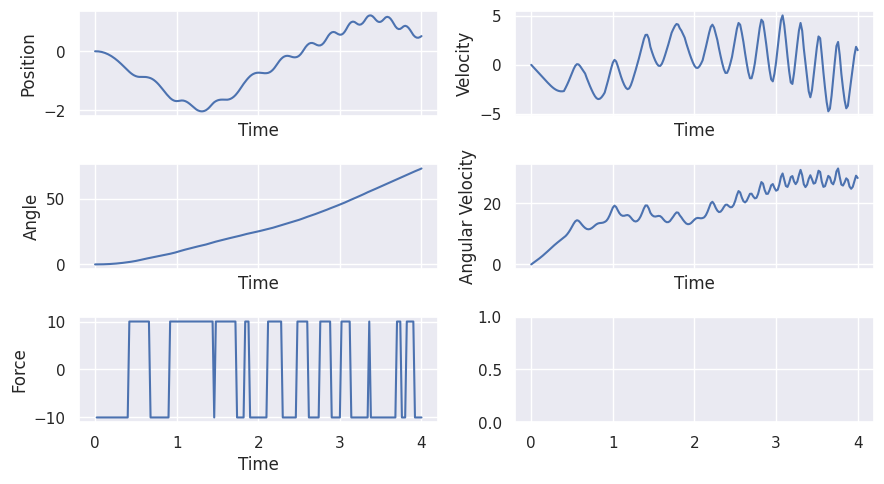
Exercise 5 (Non-Linear Inverted Pendulum MPC)
Design an MPC Controller for the non-linear inverted pendulum system for two different cases:
Cart at origin and upright Pendulum: Set the reference for the cart position to the origin.
Pendulum Swing-up: Set the initial angle to to \(-\pi\) i.e. start with the pendulum at the bottom.
Same as 2 but set the reference for the cart position to the origin.
Make the pendulum rotate as fast as possible.
Hint
Use the following to create the environment with initial angle set to -np.pi and cutoff angle to np.inf for second > case.
env = create_inverted_pendulum_environment(theta_threshold=np.inf, initial_angle=-np.pi)
Hint
You can access the inverted pendulum’s kinetic, respectively potential, energy using inverted_pendulum_lin_model.aux["E_kinetic"], respectively inverted_pendulum_lin_model.aux["E_potential"])
Solution to ( 5
Fast Rotation
We first need the environment, non-linear model and simulator:
inverted_pendulum_env = create_inverted_pendulum_environment(
    max_steps=200, theta_threshold=np.inf
)
inverted_pendulum_nonlin_model = build_inverted_pendulum_nonlinear_model(
    inverted_pendulum_env
)
inverted_pendulum_nonlin_simulator = Simulator(inverted_pendulum_nonlin_model)
inverted_pendulum_nonlin_simulator.set_param(t_step=inverted_pendulum_env.dt)
inverted_pendulum_nonlin_simulator.setup()
The goal is to make the inverted pendulum rotate as fast as possible. For that we define the following costs:
rotation_cost = -1000 * inverted_pendulum_nonlin_model.x["dtheta"]
terminal_cost = rotation_cost
stage_cost = rotation_cost
print(f"{stage_cost=}")
print(f"{terminal_cost=}")
stage_cost=SX((-1000*dtheta))
terminal_cost=SX((-1000*dtheta))
We define as well upper and lower limits for the force and position:
x_limits = {
    "position": np.array(
        [-inverted_pendulum_env.x_threshold, inverted_pendulum_env.x_threshold]
    )
}
u_limits = {
    "force": np.array(
        [-inverted_pendulum_env.force_max, inverted_pendulum_env.force_max]
    )
}
After that, we create the controller:
inverted_pendulum_mpc_controller = build_mpc_controller(
    model=inverted_pendulum_nonlin_model,
    t_step=inverted_pendulum_env.dt,
    n_horizon=50,
    stage_cost=stage_cost,
    terminal_cost=terminal_cost,
    x_limits=x_limits,
    u_limits=u_limits,
)
Simulation
Show code cell source
%%capture
inverted_pendulum_mpc_controller.reset_history()
inverted_pendulum_nonlin_simulator.reset_history()

x0 = np.random.normal(loc=np.zeros((4, 1)))
inverted_pendulum_nonlin_simulator.x0 = x0
inverted_pendulum_mpc_controller.x0 = x0
inverted_pendulum_mpc_controller.set_initial_guess()

for k in range(100):
    u0 = inverted_pendulum_mpc_controller.make_step(x0)
    x0 = inverted_pendulum_nonlin_simulator.make_step(u0)
Evaluation
class MPCController:
    def __init__(self, mpc: do_mpc.controller.MPC) -> None:
        self.mpc = mpc
        self.mpc.reset_history()
        self.mpc.x0 = np.random.normal(loc=np.zeros((4, 1)))
        self.mpc.set_initial_guess()

    def act(self, observation: NDArray) -> NDArray:
        return self.mpc.make_step(observation.reshape(-1, 1)).ravel()
Show code cell source
%%capture
mpc_controller = MPCController(inverted_pendulum_mpc_controller)
results = simulate_environment(
    inverted_pendulum_env, max_steps=200, controller=mpc_controller
)
error: XDG_RUNTIME_DIR not set in the environment.
 |
MPC Controller Design Challenges#
Some of the challenges that we are faced with when designing an MPC controller include:
Choosing the right hyper-parameters to ensure optimality as well as feasibility.
Ensuring recursive feasibility and achieving optimality despite a short prediction horizon.
Satisfying input and state constraints in the presence of uncertainty.
Ensuring computational tractability by properly reformulating constraints and costs and parameterizing control policies
Robust MPC#
Robust Model Predictive Control (RMPC) is related to a variety of methods designed to guarantee control performance using optimization algorithms while considering systems with uncertainties. It is concerned with the control of system that are only approximately known. Usually, it is assumed that the system lies in a set of possible systems and this set can be quantitatively characterized
Robust MPC guarantees constraint satisfaction for all uncertain element realizations.
The model is split into a nominal part and additive uncertainty in a compact set.
The controller is designed to be robust against the uncertainty.
The MPC cost is typically optimized for the nominal system.
Multi-Stage MPC#
The basic idea for the multi-stage approach is to consider various scenarios, where a scenario is defined by one possible realization of all uncertain parameters at every control instant within the horizon. The family of all considered discrete scenarios can be represented as a tree structure, called the scenario tree
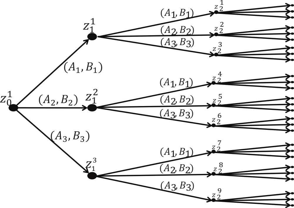
Fig. 15 Scenario tree representation of the uncertainty evolution for multi-stage MPC.#
Each node in the tree denotes the possible state of the system at every prediction step.
The branches represent the different possible realizations of the uncertainty.
The initial state of the system forms the root node of the tree.
The root node branches into several nodes in the first stage depending on the number of vertex matrix pairs of the parametric uncertainty.
All the nodes in the first stage branch again in the second stage.
The sequence continues until the end of prediction horizon N to form the complete scenario tree.
A path from the root node to the leaf node represents a scenario.
Inverted Pendulum#
In a real system, we cannot usually determine the model parameters exactly and this represents an important source of uncertainty.
In this example, we consider that the mass of the pole is not known precisely and is different from its nominal value but we know which possible values it may take.
Model#
inverted_pendulum_env = create_inverted_pendulum_environment(
    max_steps=200, theta_initial=180, theta_threshold=np.inf
)

inverted_pendulum_nonlin_model = build_inverted_pendulum_nonlinear_model(
    inverted_pendulum_env, with_uncertainty=True
)
m_p_values = inverted_pendulum_env.masspole * np.array([1.0, 1.20, 0.80])
display_array("m_p", m_p_values)
uncertainty_values = {"m_p": m_p_values}
setpoint = np.zeros((4, 1))
distance_cost = casadi.bilin(
    np.diag([1, 0, 100, 1]), inverted_pendulum_nonlin_model.x.cat - setpoint
)
terminal_cost = distance_cost
stage_cost = distance_cost
u_penalty = {"force": 1e-3}
display_array("Setpoint", setpoint)
print(f"Stage cost: {stage_cost}")
print(f"Terminal cost: {terminal_cost}")
Stage cost: ((sq(position)+((100*theta)*theta))+sq(dtheta))
Terminal cost: ((sq(position)+((100*theta)*theta))+sq(dtheta))
x_limits = {
    "position": np.array(
        [-inverted_pendulum_env.x_threshold, inverted_pendulum_env.x_threshold]
    )
}
u_limits = {
    "force": np.array(
        [-inverted_pendulum_env.force_max, inverted_pendulum_env.force_max]
    )
}
We again create an instance of MPC from the do_mpc package using the already defined build_mpc_controller function. This time however we pass the n_robust keyword argument to control the number of scenarios.
inverted_pendulum_mpc_controller = build_mpc_controller(
    model=inverted_pendulum_nonlin_model,
    t_step=inverted_pendulum_env.dt,
    n_horizon=50,
    stage_cost=stage_cost,
    terminal_cost=terminal_cost,
    x_limits=x_limits,
    u_limits=u_limits,
    u_penalty=u_penalty,
    uncertainty_values=uncertainty_values,
    n_robust=1,
)
Evaluation#
class MPCController:
    def __init__(self, mpc: do_mpc.controller.MPC) -> None:
        self.mpc = mpc
        self.mpc.reset_history()
        self.mpc.x0 = np.random.normal(loc=np.zeros((4, 1)))
        self.mpc.set_initial_guess()

    def act(self, observation: NDArray) -> NDArray:
        return self.mpc.make_step(observation.reshape(-1, 1)).ravel()
Show code cell source
%%capture
controller = MPCController(inverted_pendulum_mpc_controller)
results = simulate_environment(
    inverted_pendulum_env, max_steps=200, controller=controller
)
error: XDG_RUNTIME_DIR not set in the environment.
 |