Dynamic Programming

Dynamic programming (DP) is a method that in general solves optimization problems that involve making a sequence of decisions (multi-stage decision making problems) by determining, for each decision, subproblems that can be solved similarily, such that an optimal solution of the original problem can be found from optimal solutions of subproblems. This method is based on Bellman’s Principle of Optimality:

An optimal policy has the property that whatever the initial state and initial decision are, the remaining decisions must constitute an optimal policy with regard to the state resulting from the first decision.

A problem is said to satisfy the Principle of Optimality if the sub-solutions of an optimal solution of the problem are themselves optimal solutions for their subproblems.

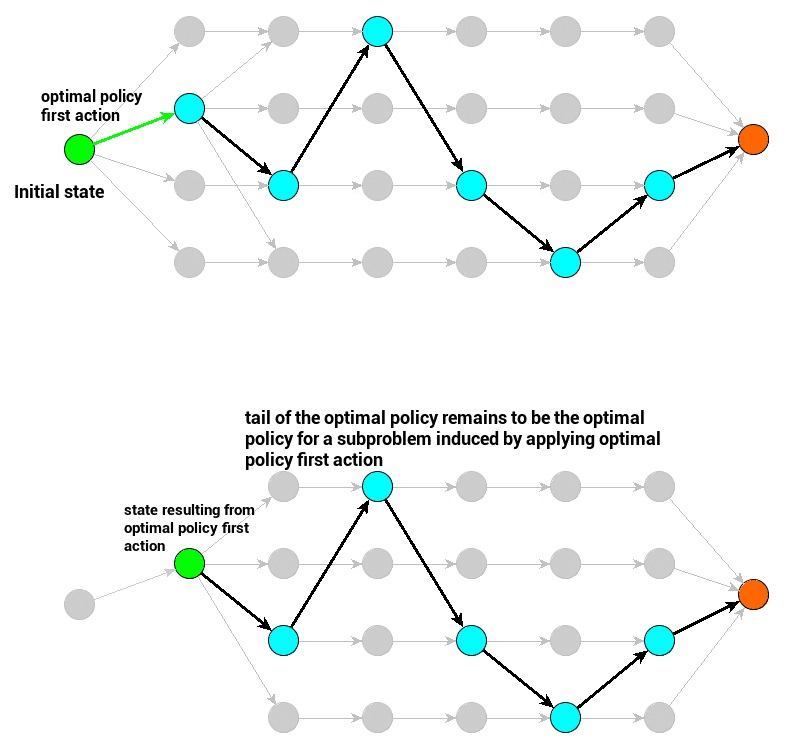
Fig. 8 Representation of optimality principle on a graph. Taken from this blog post.

• Black arrows represent sequence of optimal policy actions – the one that is evaluated with the greatest value.

• Green arrow is optimal policy first action (decision) – when applied it yields a subproblem with new initial state. Principle of optimality is related to this subproblem optimal policy.

• Green circle represents initial state for a subproblem (the original one or the one induced by applying first action)

• Red circle represents terminal state – assuming our original parametrization it is the maze exit

Usually creativity is required before we can recognize that a particular problem can be cast effectively as a dynamic program and often subtle insights are necessary to restructure the formulation so that it can be solved effectively.

Dynamic Programming is a very general solution method for problems which have these properties:

• Optimal substructure (Principle of optimality applies)

  • The optimal solution can be decomposed into subproblems, e.g., shortest path.

• Overlapping subproblems

  • The subproblems recur many times.

  • The solutions can be cached and reused.

• Additive cost function

  • The cost function along a given path can be decomposed as the sum of cost functions for each step.

It is used across a wide variety of domains, e.g.

• Scheduling algorithms

• Graph algorithms (e.g., shortest path algorithms)

• Graphical models in ML (e.g., Viterbi algorithm)

• Bioinformatics (e.g., Sequence alignment, Protein folding)

• Finance (e.g. Derivatives)

Discrete Time

We define the optimal cost-to-go function (also known as value function) for any feasible \(\mathbf{x} \in \mathbf{X}\) as[1]:

\[ V(\mathbf{x}) := \min_{u \in \mathbf{U}} J(\mathbf{x}, \mathbf{u}) \]

An admissible control sequence \(\mathbf{u}^*\) is called optimal, if

\[ V(\mathbf{x}) = J(\mathbf{x}, \mathbf{u}^*) \]

Infinite Horizon

Given the optimal cost-to-go for an infinite-horizon optimal control problem:

\[ V(\mathbf{x}_0) = \min_{\mathbf{u} \in \mathbf{U}} J(\mathbf{x}_0, \mathbf{u}) = \min_{u \in \mathbf{U}} \left[ \sum \limits_{k = 0}^{\infty} c(\mathbf{x}_k, \mathbf{u}_k) \right] \]

We can unroll the expression by one-step to obtain:

\[ V(\mathbf{x}_0) = \min_{\mathbf{u} \in \mathbf{U}} \left[ c(\mathbf{x}_0, \mathbf{u}_0) + \min_{u \in \mathbf{U}} \sum \limits_{k = 1}^{\infty} c(\mathbf{x}_k, \mathbf{u}_k) \right] \]

Which is equivalent to:

\[ V(\mathbf{x}_0) = \min_{u \in \mathbf{U}} \left[ c(\mathbf{x}_0, \mathbf{u}_0) + V(\mathbf{x}_1) \right] \]

If we now replace \(\mathbf{x}_1 = f(\mathbf{x}_0, \mathbf{u}_0)\) and then get rid of time indices we finally get:

\[ V(\mathbf{x}) = \min_{\mathbf{u} \in \mathbf{U}} \left[ c(\mathbf{x}, \mathbf{u}) + V(f(\mathbf{x}, \mathbf{u})) \right] \]

This equation is called the Bellman equation.

DP Algorithm

For every initial state \(\mathbf{x}_0\), the optimal cost is equal to \(V(\mathbf{x}_0)\), given by the last step of the following algorithm, which proceeds backward in time from stage \(N-1\) to stage \(0\):

• Start with \(V(\mathbf{x}_N) = c(\mathbf{x}_N)\)

• then for \(k = \{N - 1, \dots, 0\}\), let:

  \[ V(\mathbf{x}_k) = \displaystyle \min_{u \in \mathbf{U}} \left[ c(\mathbf{x}_k, \mathbf{u}_k) + V(f(\mathbf{x}_k, \mathbf{u}_k)) \right] \]
  \[ V(\mathbf{x}_k) = \displaystyle \min_{u \in \mathbf{U}} \left[ c(\mathbf{x}_k, \mathbf{u}_k) + V(\mathbf{x}_{k+1}) \right] \]

Once the values \(V(\mathbf{x}_0), \dots , V(\mathbf{x}_N)\) have been obtained, we can use a forward algorithm to construct an optimal control sequence \(\{u_0^*, \dots, u_{N-1}^*\}\) and corresponding state trajectory \(\{x_1^∗, \dots, x_{N}^*\}\) for the given initial state \(x_0\).

\[ \begin{equation} u^*_k = \displaystyle \underset{u \in \mathbf{U}}{\text{argmin}} \left[ c(\mathbf{x}_k, \mathbf{u}_k) + V(f(\mathbf{x}_k, \mathbf{u}_k)) \right]. \end{equation} \]

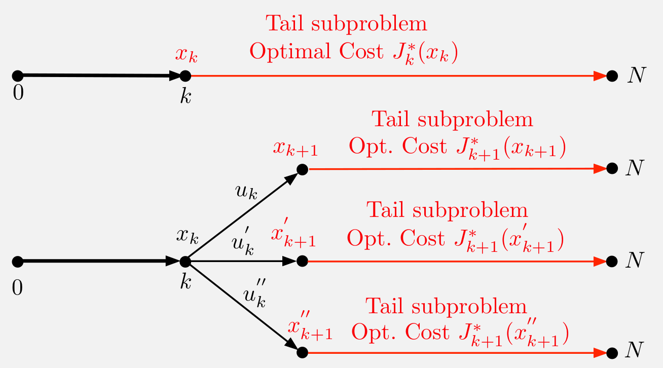
Fig. 9 Illustration of the DP algorithm. The tail subproblem that starts at \(x_k\) at time \(k\) minimizes over \(\{u_k , \dots , u_{N-1}\}\) the “cost-to-go” from \(k\) to \(N\).

Graph Search

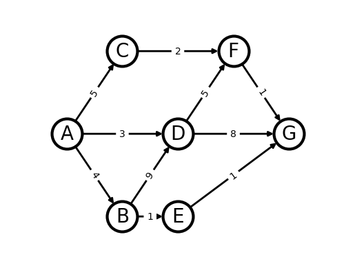
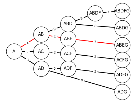
We wish to travel from node A to node G at minimum cost. If the cost represents time then we want to find the shortest path from A to G.

• Arrows (edges) indicate the possible movements.

• Numbers on edges indicate the cost of moving along an edge.

We can use Dynamic Programming to solve this problem.

We start by determining all possible paths first .

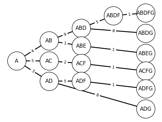
We then compute the cost-to-go at each node to determine the shortest path.

Each node in this new graph represents a state. We will start from the tail (the last states) and compute recursively the cost for each state transition.

Let \(c(n_1, n_2)\) the cost of moving from node \(n_1\) to node \(n_2\) and \(V(n)\) be the optimal cost-to-go from node \(n\).

We have \(V({\text{G}}) = 0\) because the cost of going from node \(G\) to itself is 0.

We start with nodes F and E:

\[\begin{split} \begin{array}{lll} V(\text{F}) &= c(\text{F}, \text{G}) + V({\text{G}}) &= 1 + 0 &= 1\\ V(\text{E}) &= c(\text{E}, \text{G}) + V({\text{G}}) &= 1 + 0 &= 1\\ \end{array} \end{split}\]

We then move to nodes D and C:

\[\begin{split} \begin{array}{lll} V(\text{D}) &= \min \left[ c(\text{D}, \text{G}) + V({\text{G}}), c(\text{D}, \text{F}) + V(\text{F}) \right] &= \min \left[ 8 + 0, 5 + 1 \right] &= 6 \\ V(\text{C}) &= c(\text{C}, \text{F}) + V({\text{F}}) &= 2 + 1 &= 3 \end{array} \end{split}\]

After that we move to node B:

\[ \begin{array}{lll} V(\text{B}) &= \min \left[ c(\text{B}, \text{D}) + V({\text{D}}), c(\text{B}, \text{E}) + V(\text{E}) \right] &= \min \left[ 9 + 6, 1 + 1 \right] &= 2 \end{array} \]

We finally go to node A:

\[\begin{split} \begin{array}{lll} V(\text{A}) &= \min \left[ c(\text{A}, \text{B}) + V(\text{B}), c(\text{A}, \text{C}) + V(\text{C}), c(\text{A}, \text{D}) + V(\text{D}) \right] &= \min \left[ 4 + 2, 5 + 3, 3 + 6 \right] &= 6 \\ \end{array} \end{split}\]

Now that we have computed the optimal cost-to-go, we can proceed in a forward manner to determine the best path:

\[ \pi^* = \underset{n}{\text{argmin}} [c(n_1, n_2) + V(n_2)] \]

For the first action (step) we have:

\[\begin{split} \pi^*_0 &= \underset{n_2 \in \{ B, C, D \}}{\text{argmin}} \left[ c(A, n_2) + V(n_2) \right] \\ &= \underset{n_2}{\text{argmin}} \left[ c(A, n_2 = B) + V(n_2 = B), c(A, n_2 = C) + V(n_2 = C), c(A, n_2 = D) + V(n_2 = D) \right] \\ &= \underset{n_2}{\text{argmin}} \left[ 4 + 2, 5 + 3, 3 + 6 \right] \\ &= B \end{split}\]

Proceeding the same way we get:

\[ \pi^* = \{ \pi^*_0, \pi^*_1, \pi^*_2 \} = \{ \text{B, E, G} \} \]

The shortest-path is ABEG.

Value Iteration

Another way to compute the optimal cost-to-go for all states that is also applicable is the Value Iteration algorithm:

\[\begin{split} \begin{array}{l} \textbf{Input}:\ \langle S, s_0, U, c(s, u)\rangle\\ \textbf{Output}:\ \text{Value function}\ V\\[2mm] \text{Set}\ V\ \text{to arbitrary value function; e.g., }\ V(s) = 0\ \text{for all}\ s\\[2mm] \text{repeat}\ \\ \quad\quad \Delta \leftarrow 0 \\ \quad\quad \text{foreach}\ s \in S \\ \quad\quad\quad\quad \underbrace{V'(s) \leftarrow \min_{u \in U(s)} \left[c(s, u) + \ V(s') \right]}_{\text{Bellman equation}} \\ \quad\quad\quad\quad \Delta \leftarrow \max(\Delta, |V'(s) - V(s)|) \\ \quad\quad V \leftarrow V' \\ \text{until}\ \Delta \leq 0.0 \end{array} \end{split}\]

Tip

Stochastic Value Iteration

It can also be used in stochastic systems:

\[\begin{split} \begin{array}{l} \textbf{Input}:\ \text{MDP}\ M = \langle S, s_0, U, P_u(s' \mid s), c(s, u, s')\rangle\\ \textbf{Output}:\ \text{Value function}\ V\\[2mm] \text{Set}\ V\ \text{to arbitrary value function; e.g., }\ V(s) = 0\ \text{for all}\ s\\[2mm] \text{repeat}\ \\ \quad\quad \Delta \leftarrow 0 \\ \quad\quad \text{foreach}\ s \in S \\ \quad\quad\quad\quad \underbrace{V'(s) \leftarrow \min_{u \in U(s)} \sum_{s' \in S} P_a(s' \mid s)\ [c(s,a,s') + \gamma\ V(s') ]}_{\text{Bellman equation}} \\ \quad\quad\quad\quad \Delta \leftarrow \max(\Delta, |V'(s) - V(s)|) \\ \quad\quad V \leftarrow V' \\ \text{until}\ \Delta \leq \theta \end{array} \end{split}\]

Optimal Control as Graph Search

We can formulate discrete-time optimal control problems as graph search problems by either considering a system with discrete states and actions or by discretizing a system with continuous states and actions.

Exercise

Exercise 2 (Grid World)

Show code cell source Hide code cell source

env = create_grid_world_environment(render_mode="rgb_array", max_steps=50)
result = simulate_environment(env)
show_video(result.frames, fps=3)

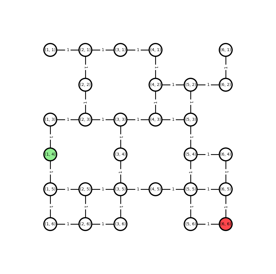
The task can be represented as the following undirected graph:

Show code cell source Hide code cell source

env.reset()
G = env.unwrapped.get_graph()
plot_grid_graph(G)

We convert the graph to a directed graph with all possible paths from start to target that do not contain cycles

Show code cell source Hide code cell source

G = convert_graph_to_directed(G)
plot_grid_graph(G)

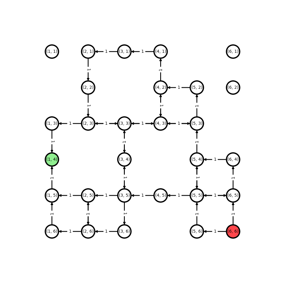
We wish for the car to travel from its starting cell in red to the target cell in green. If the cost represents time and each step has the same cost then we want to find the shortest path to the goal.

• Arrows (edges) indicate the possible movements.

• Numbers on edges indicate the cost of moving along an edge.

Use Dynamic Programming to solve this problem:

• Determine the number of possible paths from start position to target position.

• Compute the optimal cost-to-go for each state.

• Determine the optimal plan using the computed optimal cost-to-go.

• Implement the plan in the environment.

Tip

Hint 1

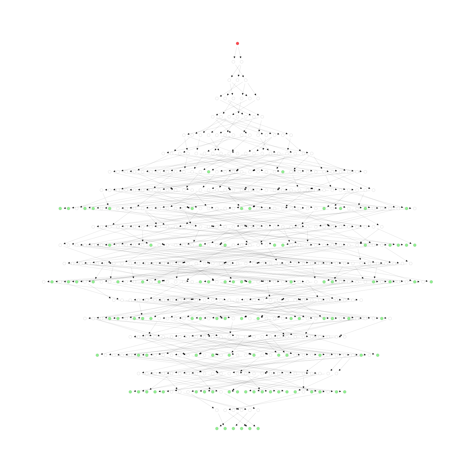
Determine all possible paths first.

You can use plot_grid_all_paths_graph(G) for that.

Tip

Hint 2

Compute the optimal cost-to-go at each node.

You can use dict(G.nodes(data=True)) to get a dictionary that maps the nodes to their attributes and you can use G.start_node and G.target_node to access the start and target nodes, respectively.

Solution to ( 2

For this solution we first need to import some functions:

from training_ml_control.environments import (
    value_iteration,
    compute_best_path_and_actions_from_values,
)
import networkx as nx

To determine the number of paths from start node to target node we use:

len(
    list(
        nx.all_simple_paths(
            G.to_undirected(), source=G.start_node, target=G.target_node, cutoff=len(G)
        )
    )
)

101

After that, to plot all paths from start to end we use:

plot_grid_all_paths_graph(G)

To compute the optimal cost-to-go we use:

values = value_iteration(G)

Once that’s computed, we can determine the best path and correponding actions:

best_path, actions = compute_best_path_and_actions_from_values(
    G, start_node=G.start_node, target_node=G.target_node, values=values
)
print(f"{best_path=}")
print(f"{actions=}")

best_path=[(6, 6), (6, 6), (5, 6), (5, 5), (4, 5), (3, 5), (2, 5), (1, 5)]
actions=[2, 3, 2, 2, 2, 2, 3]

We finally apply the computed plan to the environment and check that it indeed works:

env.reset()
for action in actions:
    observation, _, terminated, truncated, _ = env.step(action)
    if terminated or truncated:
        frames = env.render()
        env.reset()
        break
env.close()
show_video(frames, fps=3)

Continuous Time

Let’s consider a continuous-time optimal control problem with finite horizon over the time period \([t_0 ,t_f]\).

The system’s dynamics is given by:

\[ \dot{\mathbf{x}}(t) = f(\mathbf{x}(t), \mathbf{u}(t)) \]

With the initial state \(\mathbf{x}(t_0) = \mathbf{x}_0\)

The cost-to-go is given by:

\[ J(\mathbf{x}(t), \mathbf{u}(t), t_0, t_f) = c_f(\mathbf{x}(t_f), t_f) + \int\limits_{t_0}^{t_f} c(\mathbf{x}(t), \mathbf{u}(t)) d\tau \]

The optimal cost-to-go is given by:

\[ \displaystyle V(\mathbf{x}(t), t_0, t_f) = \underset{\mathbf{u(t)}}{min} \left[ J(\mathbf{x}(t), \mathbf{u}(t), t_0, t_f) \right] \]

It can be show that for every \(s, \tau \in [t_0, t_f]\), \(s \leq \tau\) , and \(\mathbf{x} \in \mathbf{X}\), we have:

\[ V(s, \mathbf{x}) = \underset{\mathbf{u(t)}}{min} \left[ \int\limits_{s}^{\tau} c(\mathbf{x}(t), \mathbf{u}(t)) d\tau + V(\tau, \mathbf{x}(\tau)) \right] \]

Which is another version of the Bellman equation.

Hamilton-Jacobi-Bellman Equation

The Hamilton-Jacobi-Bellman (HJB) equation is given by:

\[ - \frac{\partial V}{\partial t} = \underset{\mathbf{u(t)}}{min} \left[ \left( \frac{\partial V}{\partial \mathbf{x}} \right)^T f(\mathbf{x}(t), \mathbf{u}(t)) + c(\mathbf{x}(t), \mathbf{u}(t)) \right] \]

It is a sufficient condition of optimality i.e., that if \(V\) satisfies the HJB, it must be the value function.

---

[1]

for the sake of simplicity we will focus on the discrete-time case