Machine Learning & Control

Modern machine learning provides useful tools and perspectives for control theory. Framing control problems as data modeling tasks enables powerful function approximation, estimation, and optimization techniques from machine learning to be applied.

Learning-Based Control

• Learning-based control addresses the automated and data-driven generation or adaptation of elements of the controller formulation to improve control performance.

• The learning setup can be diverse:

  • Offline learning involves adapting the controller between trials or episodes while collecting data.

  • Online learning adjusts the controller during closed-loop operation (e.g. repetitive tasks) or using data from one task execution.

System Identification

System Identification is the process of constructing a model of a (dynamical) system from observations (measurements) of its inputs and outputs. System identification also includes the optimal design of experiments for efficiently generating informative data for fitting such models as well as model reduction.

In control engineering, the objective is to obtain a good performance of the closed-loop system, which is the one comprising the physical system, the feedback loop and the controller. This performance is typically achieved by designing the control law relying on a model of the system, which needs to be identified starting from experimental data. If the model identification procedure is aimed at control purposes, what really matters is not to obtain the best possible model that fits the data, as in the classical system identification approach, but to obtain a model satisfying enough for the closed-loop performance.

In control engineering, we typically rely on the mathematical modelling of the system from first principles and then optionally use parameter identification methods to determine the values of the mathematical model’s parameters.

In our case, we will not rely on that and instead prefer fitting a model based only on measured data.

Exercise 6 (Dynamic System Model Evaluation)

How do we evaluation the fitted model of the system?

Solution to ( 6

• We could evaluate the model’s prediction on a held-out validation set.

• Additionally we could evaluate the model’s long-term predictions in an open-loop manner.

• On top of that, we could evaluate the model’s step[1] and impulse[2] responses from different initial states. This is especially useful for linear systems.

• It is also valuable to look at what the model’s residuals and make sure there is no correlation with other available information such as the input.

Data Collection

Before learning a model of the system, we need to collect either during the system’s operation i.e. online data collection, or inbetween episodes of the system’s operation i.e. offline data collection. The collected data has to be informative, i.e. comprehensive and be representative of the all behaviours of the system that we desire to capture.

Data informativity is a condition on the data under which it is possible to distinguish between different models in a (parametric) model class.

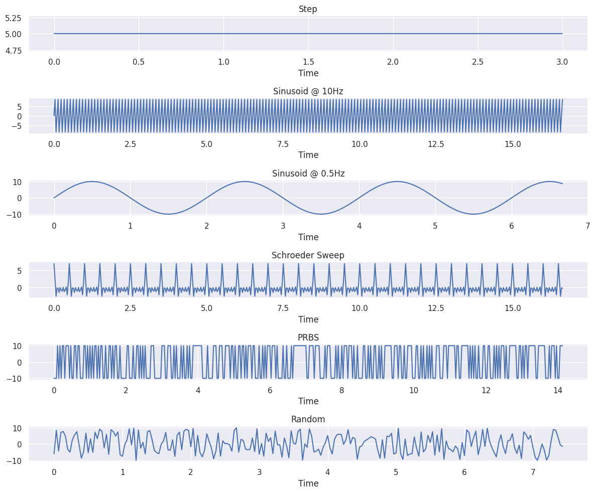
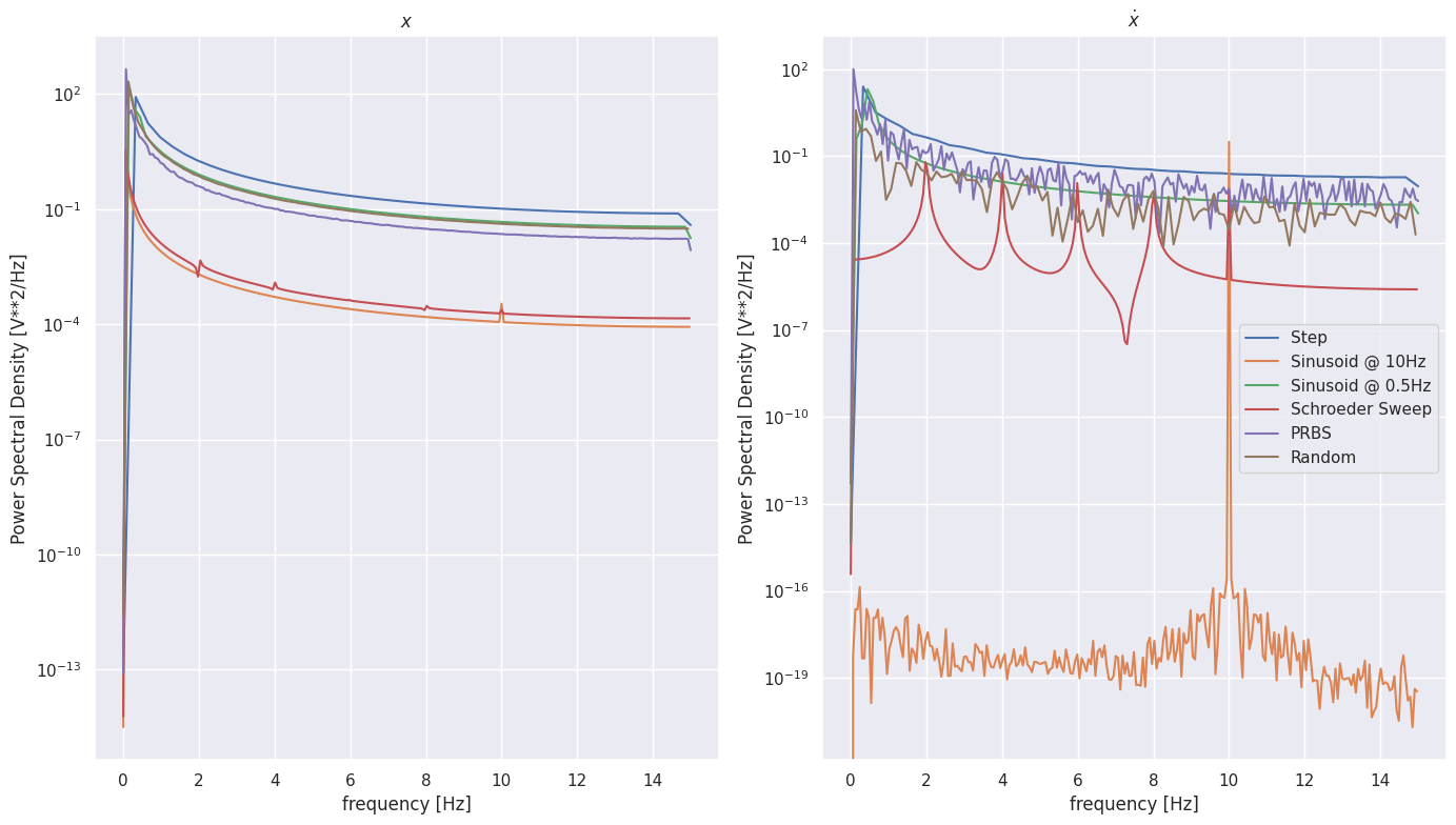
Commonly used input signals for system identification:

• Step function

• Pseudorandom binary sequence (PRBS)

• Autoregressive, moving average process

• Periodic signals: sum of sinusoids

• Schroeder Sweep (Sum of phase shifted sinusoids)

  \[ u(t) = \sum\limits_{k=1}^M A_k \cos(\frac{2\pi k \tau(t)}{T} + \phi_k), \quad t = 0, 1, \dots , N − 1 \]

  Where:

  \[\begin{split} \begin{array}{l} k = \sqrt{\frac{P}{M}}\\ \phi_1 = 0\\ \phi_k = \phi_{k-1} − \frac{\pi k^2}{N}, \quad k = 2, 3, \dots , M \end{array} \end{split}\]

  With \(M\) the number of harmonically related frequencies, \(\phi_k\) the phase angles of the harmonic components to produce low Peak Factor (PF), \(N\) the number of time steps, \(P\) the total desired input power.

For certain systems in many safety-critical tasks such as space exploration or robot-assisted surgery we have to rely on human experts to control the system and avoid damaging it or its environment.

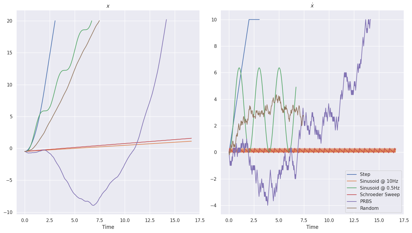
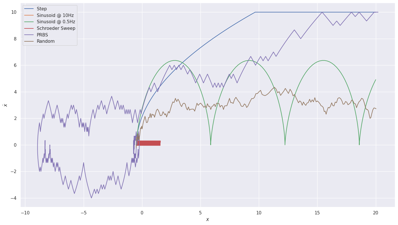
Cart

cart_env = create_cart_environment(max_steps=500, goal_position=20, max_position=30)

Show code cell content Hide code cell content

cart_observations = {}
cart_actions = {}
cart_frames = {}

controllers = {
    "Step": ConstantController(np.asarray([cart_env.max_action / 2])),
    "Sinusoid @ 10Hz": SineController(
        cart_env, np.asarray([cart_env.max_action]), frequency=10
    ),
    "Sinusoid @ 0.5Hz": SineController(
        cart_env, np.asarray([cart_env.max_action]), frequency=0.5
    ),
    "Schroeder Sweep": SchroederSweepController(
        cart_env,
        n_time_steps=500,
        n_harmonics=5,
        frequency=2,
    ),
    "PRBS": PRBSController(np.asarray([cart_env.max_action])),
    "Random": RandomController(cart_env),
}

for controller_name, controller in controllers.items():
    result = simulate_environment(cart_env, controller=controller)
    cart_observations[controller_name] = result.observations
    cart_actions[controller_name] = result.actions
    cart_frames[controller_name] = result.frames

error: XDG_RUNTIME_DIR not set in the environment.

Let’s look at the phase portrait[3] instead.

Let’s visualize the Power Spectral Density (PSD) of the input and state signals

Model Fitting

Naive Deep Learning

\[ \mathbf{x}_{t+1} = f_\theta(\mathbf{x}_t, \mathbf{u}_t) \]

Where \(\theta\) are learnable parameters.

Issues with such an approach:

• Domain shift from the training distribution to the real-world distribution.

• Black-box.

Deep Learning with Nominal Model

A real-world dynamical system can be described as:

\[ \mathbf{x}_{t+1} = \underbrace{f_n(\mathbf{x}_t, \mathbf{u}_t)}_{\text{nominal dynamics}} + \underbrace{g_r(\mathbf{x}_t, \mathbf{u}_t)}_{\text{residual dynamics}} + \underbrace{w_t}_{\text{disturbance}} \]

Where \(f_n\) is the nominalsystem model, \(g_r\) an additive residual term accommodating uncertainty and \(w_t\) represents distburnances.

Many learning-based techniques make use of this explicit distinction by only learning the residual term.

An example of the use of this approach can be found in [SSOConnell+19].

Visual depiction of the ground effect, the complex aerodynamic effect between the drone and the ground, which is nonlinear, nonstationary, and very hard to model using standard system identification approaches. Adapted from Neural Control blog post. is a figure depicting the ground effect that is modelled using a neural network and Comparison of drone landing with and without neural network modelling of residual ground effect. Taken from Neural Control blog post. is a comparison of drone landings with and without neural network modeling.

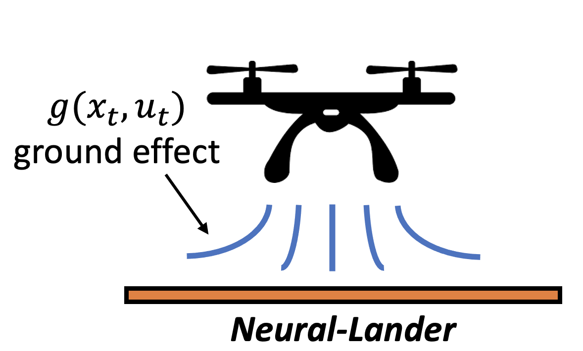
Fig. 17 Visual depiction of the ground effect, the complex aerodynamic effect between the drone and the ground, which is nonlinear, nonstationary, and very hard to model using standard system identification approaches. Adapted from Neural Control blog post.

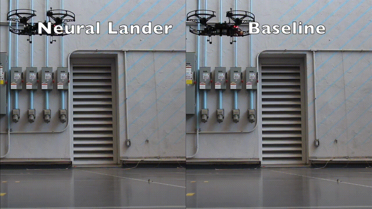
Fig. 18 Comparison of drone landing with and without neural network modelling of residual ground effect. Taken from Neural Control blog post.

Issues with such an approach:

• Requires nominal model.

• Still susceptible to domain shift issues.

Sparse Identification of Nonlinear Dynamics (SINDy)

The SINDY algorithm identifies fully nonlinear dynamical systems from measurement data. This relies on the fact that many dynamical systems have relatively few terms in the right hand side of the governing equations:

\[ \dot{\mathbf{x}} = f(\mathbf{x}) \]

To determine the function \(f\) from data, we collect a time history of the state \(\mathbf{x}\) and either measure the derivative \(\dot{\mathbf{x}}\) or approximate it numerically. The data are sampled at several times \(t_1, t_2, \dots, t_m\) and arranged into two matrices:

\[\begin{split} \mathbf{X} = \begin{bmatrix} \mathbf{x}^T(t_1)\\ \mathbf{x}^T(t_2)\\ \vdots\\ \mathbf{x}^T(t_m) \end{bmatrix} = \begin{bmatrix} x_1(t_1) & x_2(t_1) & \dots & x_n(t_1)\\ x_1(t_2) & x_2(t_2) & \dots & x_n(t_2)\\ \vdots & \vdots & \ddots & \vdots\\ x_1(t_m) & x_2(t_m) & \dots & x_n(t_m)\\ \end{bmatrix} \end{split}\]

\[\begin{split} \dot{\mathbf{X}} = \begin{bmatrix} \dot{\mathbf{x}}^T(t_1)\\ \dot{\mathbf{x}}^T(t_2)\\ \vdots\\ \dot{\mathbf{x}}^T(t_m) \end{bmatrix} = \begin{bmatrix} \dot{x}_1(t_1) & \dot{x}_2(t_1) & \dots & \dot{x}_n(t_1)\\ \dot{x}_1(t_2) & \dot{x}_2(t_2) & \dots & \dot{x}_n(t_2)\\ \vdots & \vdots & \ddots & \vdots\\ \dot{x}_1(t_m) & \dot{x}_2(t_m) & \dots & \dot{x}_n(t_m)\\ \end{bmatrix} \end{split}\]

Next, we construct a library \(\Theta(\mathbf{X})\) consisting of candidate non-linear functions of the columns of \(\mathbf{X}\). For example, \Theta(\mathbf{X})$ may consist of constant, polynomial, and trigonometric terms:

\[ \Theta(\mathbf{X}) = \begin{bmatrix} \mathbf{1} & \mathbf{X} & \mathbf{X}^{P_2} & \mathbf{X}^{P_3} & \dots & \sin(\mathbf{X}) & \cos(\mathbf{X}) \end{bmatrix} \]

Here, higher polynomials are denoted as \(\mathbf{X}^{P_2}\), \(\mathbf{X}^{P_3}\), etc., where \(\mathbf{X}^{P_2}\) denotes the quadratic nonlinearities in the state x:

\[\begin{split} \mathbf{X}^{P_2} = \begin{bmatrix} x_1^2(t_1) & x_1(t_1)x_2(t_1) & \dots & x_n^2(t_1)\\ x_1^2(t_2) & x_1(t_2)x_2(t_2) & \dots & x_n^2(t_2)\\ \vdots & \vdots & \ddots & \vdots\\ x_1^2(t_m) & x_1(t_m)x_2(t_m) & \dots & x_n^2(t_m)\\ \end{bmatrix} \end{split}\]

Each column of \(\Theta(\mathbf{X})\) represents a candidate function for the right-hand side of the system’s ODE. There is tremendous freedom in choosing the entries in this matrix of nonlinearities.

Because we assume that only a few of these nonlinearities are active in each row of \(f\), we may set up a sparse regression problem to determine the sparse vectors of coefficients \(\Xi = \begin{bmatrix} \xi_1 ^ \xi_2 & \dots & \xi_n \end{bmatrix}\) that determine which nonlinearities are active:

\[ \dot{\mathbf{X}} = \Theta(\mathbf{X})\Xi \]

This is illustrated in Schematic of the SINDy algorithm, demonstrated on the Lorenz equations. Data are collected from the system, including a time history of the states \mathbf{X} and derivatives \dot{\mathbf{X}}. Next, a library of nonlinear functions of the states, \Theta(\mathbf{X}), is constructed. This is then used to find the fewest terms needed to satisfy \dot{\mathbf{X}} = \Theta(\mathbf{X})\Xi. The few entries in the vectors of \Xi, solved for by sparse regression, denote the relevant terms in the right-hand side of the dynamics. Taken from brunton_discovering_2016. Each column \(\xi_k\) of \(Xi\) is a sparse vector of coefficients determining which terms are active in the right-hand side for one of the row equations:

\[ \dot{x}_k = f_k(x) = \Theta(x^T)\xi_k \]

Fig. 19 Schematic of the SINDy algorithm, demonstrated on the Lorenz equations. Data are collected from the system, including a time history of the states \(\mathbf{X}\) and derivatives \(\dot{\mathbf{X}}\). Next, a library of nonlinear functions of the states, \(\Theta(\mathbf{X})\), is constructed. This is then used to find the fewest terms needed to satisfy \(\dot{\mathbf{X}} = \Theta(\mathbf{X})\Xi\). The few entries in the vectors of \(\Xi\), solved for by sparse regression, denote the relevant terms in the right-hand side of the dynamics. Taken from [BPK16a]

SINDy with Control (SINDyc)

SINDYc generalizes the SINDY method to include inputs and control. In particular, it considers the nonlinear dynamical system with inputs \(\mathbf{u}\):

\[ \dot{\mathbf{x}} = f(\mathbf{x}, \mathbf{u}) \]

The SINDY algorithm is readily generalized to include actuation, as this merely requires building a larger library \(\Theta(\mathbf{X}, \mathbf{U})\) of candidate functions that include \(u\); these functions can include nonlinear cross terms in \(\mathbf{x}\) and \(\mathbf{u}\). This extension requires measurements of the state \(\mathbf{x}\) as well as the input signal \(\mathbf{u}\).

Fig. 20 Schematic of the SINDy with control algorithm. Active terms in a library of candidate nonlinearities are selected via sparse regression. Taken from [FKK+21].

Koopman Operator

Fig. 21 Summary of the idea of Koopman operators. By lifting to a space of observables, we trade a nonlinear finite-dimensional system for a linear infinite-dimensional system. Taken from [Col23].

Given \(\mathcal{F}\) a space of functions \(g: \Omega \rightarrow \mathbb{C}\), and \(\Omega\) the state space of our dynamical system. The Koopman operator is defined on a suitable domain \(\mathcal{D}(\mathcal{K}) \subset \mathcal{F}\) via the composition formula:

\[ [\mathcal{K}g](\mathbf{x}) = [g \circ f](\mathbf{x}) = g(f(\mathbf{x})), \quad g \in \mathcal{D}(\mathcal{K}) \]

Where \(\mathbf{x}_{t+1} = f(\mathbf{x}_t)\)

The functions \(g\), referred to as observables, serve as tools for indirectly measuring the state of the system. Specifically, \(g(x_t)\) indirectly measures the state \(x_t\).

In this context, \([\mathcal{K}g](\mathbf{x}_t) = g(f(\mathbf{x}_t)) = g(\mathbf{x}_{t+1})\) represents the measurement of the state one time step ahead of \(g(\mathbf{x}_t)\). This process effectively captures the dynamic progression of the system.

The key property of the Koopman operator \(\mathcal{K}\) is its linearity. This linearity holds irrespective of whether the system’s dynamics are linear or nonlinear. Consequently, the spectral properties of \(\mathcal{K}\) become a powerful tool in analyzing the dynamical system’s behavior.

if \(g \in \mathcal{F}\) is an eigenfunction of \(\mathcal{K}\) with eigenvalue \(\lambda\), then:

\[ g(\mathbf{x}_t) = [\mathcal{K}^t g](\mathbf{x}_0) = λ^t g(\mathbf{x}_0), \quad \forall n \in \mathbb{N}. \]

One of the most useful features of Koopman operators is the Koopman Mode Decomposition (KMD). The KMD expresses the state \(\mathbf{x}\) or an observable \(g(\mathbf{x})\) as a linear combination of dominant coherent structures. It can be considered a diagonalization of the Koopman operator.

As a result, the KMD is invaluable for tasks such as dimensionality and model reduction. It generalizes the space-time separation of variables typically achieved through the Fourier transformor singular value decomposition (SVD).

Dynamic Mode Decomposition (DMD)

Dynamic Mode Decomposition (DMD) is a popular data-driven analysis technique used to decompose complex, nonlinear systems into a set of coherent structures (also called DMD modes), that grow, decay, and/or oscillate in time revealing underlying patterns and dynamics through spectral analysis. In other words, the DMD converts a dynamical system into a superposition of modes whose dynamics are governed by eigenvalues.

The simplest and historically first interpretation of DMD is as a linear regression.

We consider a discrete-time dynamical systems represented as:

\[ \mathbf{x}_{t+1} = f(\mathbf{x}_t), \quad n = 0, 1, 2, \dots, \]

Given discrete-time snapshots of the system:

\[ \{\mathbf{x}^{(m)}, \mathbf{y}^{(m)}\}^M_{m=1}, \quad \text{s.t.} \quad \mathbf{y}^{(m)} = f(\mathbf{x}^{(m)}), \quad m = 1, \dots , M. \]

We define the snapshot matrices \(\mathbf{X}, \mathbf{Y} \in \mathbb{C}^{d\times M}\) as:

\[ \mathbf{X} = \begin{bmatrix}x^{(1)} & x^{(2)} & \dots & x^{(M)} \end{bmatrix} \]

\[ \mathbf{Y} = \begin{bmatrix}y^{(1)} & y^{(2)} & \dots & y^{(M)} \end{bmatrix} \]

We seek a matrix \(\mathbf{K}_{\text{DMD}}\) such that \(\mathbf{Y} \approx \mathbf{K}_{\text{DMD}} \mathbf{X}\). We can think of this as constructing a linear and approximate dynamical system.

To find a suitable matrix KDMD, we consider the minimization problem:

(1)\[ \underset{\mathbf{K}_{\text{DMD}} \in \mathbb{C}^{d\times d} }{\min} \left\lVert \mathbf{Y} − \mathbf{K}_{\text{DMD}} \mathbf{X} \right\rVert_F , \]

where \(\left\lVert . \right\rVert_F\) denotes the Frobenius norm[4]. Similar optimization problems will be at the heart of the various DMD-type algorithms we consider in this review. A solution to the problem in (1) is:

\[ \mathbf{K}_{\text{DMD}} = \mathbf{Y} \mathbf{X}^{+} ∈ \mathbb{C}^{d\times d}, \]

where \(^{+}\) denotes the Moore–Penrose pseudoinverse.

In practice, this is computed using the Singular Value Decomposition (SVD) as follows:

\[\begin{split} \begin{array}{ll} \mathbf{X} \approx U \Sigma V^∗ & \text{(truncated SVD of rank r)}\\ \tilde{\mathbf{K}}_{\text{DMD}} = U^∗\mathbf{Y} V \Sigma^{-1} & \text{(Compute compression)}\\ \tilde{\mathbf{K}}_{\text{DMD}} W = W \Lambda & \text{(Compute eigendecomposition)}\\ \phi = YV\Sigma^{-1}W & \text{(Compute the modes)}\\ \end{array} \end{split}\]

The core goal of DMD is to apply linear algebra and spectral techniques to the analysis, prediction, and control of nonlinear dynamical systems. However, DMD often faces several challenges that have been a driving force for the many versions of the DMD algorithm that have appeared.

Generally speaking, the error of DMD and its approximate KMD can be split into three types:

• The projection error is due to projecting/truncating the Koopman operator onto a finite-dimensional space of observables. This is linked to the issue of closure and lack of (or lack of knowledge of) non-trivial finite-dimensional Koopman invariant subspaces.

• The estimation error is due to estimating the matrices that represent the projected Koopman operator from a finite set of potentially noisy trajectory data.

• Numerical errors (e.g., roundoff, stability, further compression, etc.) incurred when processing the finite DMD matrix.

Variants

Table 1 Summary of some DMD methods. Adapted from [Col23].

DMD Method	Challenges Overcome	Key Insight/Development
Forward-Backward DMD	Sensor noise bias.	Take geometric mean of forward and backward propagators for the data.
Total Least-Squares DMD	Sensor noise bias.	Replace least-squares problem with total least-squares problem.
Optimized DMD Bagging Optimized DMD	Sensor noise bias. Optimal collective processing of snapshots.	Exponential fitting problem, solve using variable projection method. Statistical bagging sampling strategy.
Compressed Sensing	Computational efficiency. Temporal or spatial undersampling.	Unitary invariance of DMD extended to settings of compressed sensing (e.g., RIP, sparsity-promoting regularizers).
Randomized DMD	Computational efficiency. Memory usage.	Sketch data matrix for computations in reduced-dimensional space.
Multiresolution DMD	Multiscale dynamics.	Filtered decomposition across scales.
DMD with Control	Separation of unforced dynamics and actuation.	Generalized regression for globally linear control framework.
Extended DMD	Nonlinear observables.	Arbitrary (nonlinear) dictionaries, recasting of DMD as a Galerkin method.
Physics-Informed DMD	Preserving structure of dynamical systems. Numerous instances given in general framework.	Restrict the least-squares optimization to lie on a matrix manifold.

DMD with Control (DMDc)

Fig. 22 Overview of Dynamic Mode Decomposition with Control (DMDc). Adapted from [PBK16].

One of the most successful applications of the Koopman operator framework lies in control with demonstrated successes in various challenging appli- cations. These include fluid dynamics, robotics, power grids, biology, and chemical processes.

The key point is that Koopman operators represent nonlinear dynamics within a globally linear framework. This approach leads to tractable convex optimization problems and circumvents theoretical and computational limitations associated with nonlinearity. Moreover, it is amenable to data-driven, model-free approaches.

DMDc extends DMD to disambiguate between unforced dynamics and the effect of actuation.

The DMD regression is generalized to:

\[ \mathbf{x}_{t+1} = f(\mathbf{x}_t, \mathbf{u}_t) \approx A \mathbf{x}_t + B \mathbf{u}_t \]

where \(A \in \mathbb{C}^{d\times d}\) and $B \in \mathbb{C}^{d\times q} are unknown matrices.

Snapshot triplets of the form \(\{\mathbf{x}^{(m)}, \mathbf{y}^{(m)}, \mathbf{u}^{(m)}\}^M_{m=1}\) are collected, where we assume that:

\[ \mathbf{y}^{(m)} \approx f(\mathbf{x}^{(m)}, \mathbf{u}^{(m)}), \quad m = 1, \dots , M. \]

The control portion of the snapshots is arranged into the matrix \(\Upsilon = \begin{pmatrix}u^{(1)} & u^{(2)} & \dots & u^{(M)}\end{pmatrix}\).

The optimization problem in (1) is replaced by

(2)\[\begin{split} \underset{A, B}{\min} \left\lVert \mathbf{Y} − \begin{pmatrix}A & B \end{pmatrix}\Omega \right\rVert_F^2,\\ \text{where} \quad \Omega = \begin{pmatrix}\mathbf{X} \\ \Upsilon\end{pmatrix} \end{split}\]

A solution is given as \(\begin{pmatrix}A & B \end{pmatrix} = \mathbf{Y} \Omega^{+}\).

Comparison

Fig. 23 Overview of various methods that use regression to identify dynamics from data. Taken from [BPK16b].

Application to Systems

Cart

We will use the DMDc and the SINDYc methods to fit a model on the data collected from the Cart environment.

Data

Show code cell content Hide code cell content

cart_env = create_cart_environment(max_steps=500, goal_position=29, max_position=30)

cart_observations = {}
cart_actions = {}

controllers = {
    "Step": ConstantController(np.asarray([cart_env.max_action / 2])),
    "Schroeder Sweep": SchroederSweepController(
        cart_env,
        n_time_steps=500,
        n_harmonics=5,
        frequency=2,
    ),
    "PRBS": PRBSController(np.asarray([cart_env.max_action])),
}

for controller_name, controller in controllers.items():
    result = simulate_environment(cart_env, controller=controller)
    cart_observations[controller_name] = result.observations
    cart_actions[controller_name] = result.actions

error: XDG_RUNTIME_DIR not set in the environment.

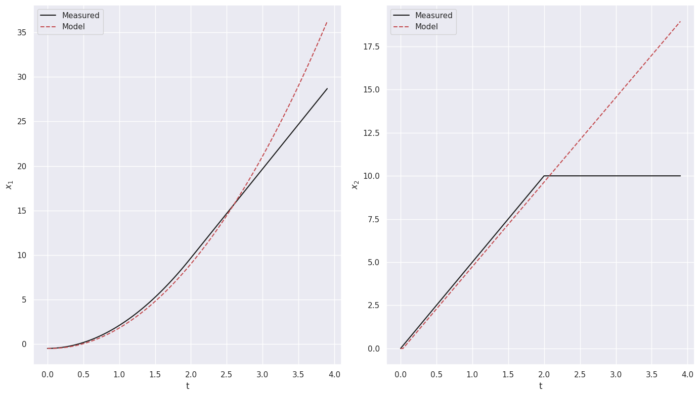
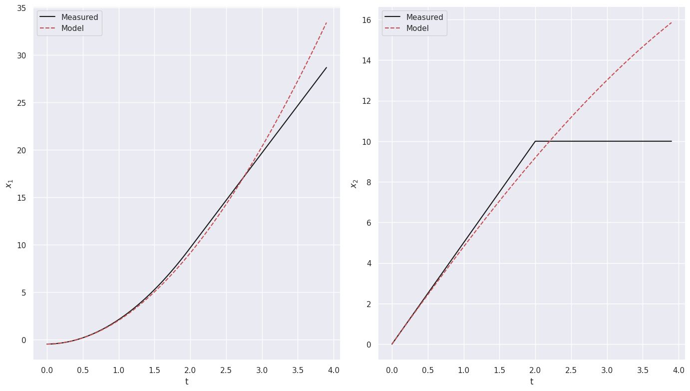
We use the data from the PRBS controller as training data and use the one from the Step controller as validation data.

training_controller_name = "PRBS"
testing_controller_name = "Step"

X_train = cart_observations[training_controller_name][:-1].copy()
U_train = cart_actions[training_controller_name].copy()
t_train = np.arange(0, len(X_train)) * cart_env.dt

X_val = cart_observations[testing_controller_name][:-1].copy()
U_val = cart_actions[testing_controller_name].copy()
t_val = np.arange(0, len(X_val)) * cart_env.dt

SINDYc

For the SINDYc method we use the pysindy package.

Refer to its introduction page for usage information.

We define an optimizer, a feature library and a differentiation method with appropriate hyper-parameters and then fit the model on the training data

optimizer = ps.STLSQ(threshold=0.1, max_iter=100)
feature_library = ps.IdentityLibrary()
differentiation_method = ps.FiniteDifference(order=1)
sindy_model = ps.SINDy(
    optimizer=optimizer,
    feature_library=feature_library,
    differentiation_method=differentiation_method,
)
sindy_model.fit(X_train, u=U_train, t=t_train)

SINDy(differentiation_method=FiniteDifference(order=1),
      feature_library=<pysindy.feature_library.identity_library.IdentityLibrary object at 0x7ff73ef01d80>,
      feature_names=['x0', 'x1', 'u0'], optimizer=STLSQ(max_iter=100))

In a Jupyter environment, please rerun this cell to show the HTML representation or trust the notebook.
On GitHub, the HTML representation is unable to render, please try loading this page with nbviewer.org.

Once that’s done, we can print the fitted model

(x0)' = 1.002 x1
(x1)' = 0.980 u0

We can also compute a score for the fitted model.

By default this is computes the \(R^2\) score[5], also called coefficient of determination, but we will instead using the Mean Squared Error metric.

Model score: 5.911230

Let us now use the model to simulate the system’s response with the test inputs and as initial state the first state in the test data

Show code cell content Hide code cell content

X_sindy = sindy_model.simulate(X_val[0], t_val, u=U_val)
X_sindy = np.vstack([X_val[0][np.newaxis, :], X_sindy])

DMDc

For the DMDc method we use the pykoopman package.

Refer to its documentation page for usage information.

We start by defining a regression method, DMDs in this case, with appropriate hyper-parameters.

Afterwards we use that to create and then fit a model on the training data.

DMDc = pk.regression.DMDc(svd_output_rank=4, svd_rank=6)
dmd_model = pk.Koopman(regressor=DMDc)
dmd_model.fit(X_train, u=U_train, dt=cart_env.dt)

Koopman(observables=Identity(), regressor=DMDc(svd_output_rank=4, svd_rank=6))

In a Jupyter environment, please rerun this cell to show the HTML representation or trust the notebook.
On GitHub, the HTML representation is unable to render, please try loading this page with nbviewer.org.

Once we fit the model we can access the linear state-space models matrices:

\[\begin{split}\displaystyle \begin{equation*}A = \begin{bmatrix}1.010510751239029 &-0.02863348988997971 \\0.006065974861300678 &0.9879637714484827 \\\end{bmatrix}\end{equation*}\end{split}\]

\[\begin{split}\displaystyle \begin{equation*}B = \begin{bmatrix}-0.01287051854881282 \\0.030159189580408505 \\\end{bmatrix}\end{equation*}\end{split}\]

\[\begin{split}\displaystyle \begin{equation*}C = \begin{bmatrix}-0.9323152899742126 &-0.36164650321006775 \\-0.36164650321006775 &0.9323152899742126 \\\end{bmatrix}\end{equation*}\end{split}\]

\[\begin{split}\displaystyle \begin{equation*}W = \begin{bmatrix}(-0.9762558892999682+0.0783197876731853j) &(-0.9762558892999682-0.0783197876731853j) \\(0.0049251618999634345-0.20190637793290236j) &(0.0049251618999634345+0.20190637793290236j) \\\end{bmatrix}\end{equation*}\end{split}\]

These matrices are different from the ones that we used in our model previously because they are acting on measurements and not on the actual states.

After that we can use the model to simulate the system using the test data.

X_dmd = dmd_model.simulate(X_val[0], U_val, n_steps=X_val.shape[0] - 1)
X_dmd = np.vstack([X_val[0][np.newaxis, :], X_dmd])

/opt/conda/lib/python3.10/site-packages/pykoopman/koopman.py:302: ComplexWarning: Casting complex values to real discards the imaginary part
  x = x.astype(self.A.dtype)

We can also compute score similarily to what we did for SINDyc

Model score: 3.758127

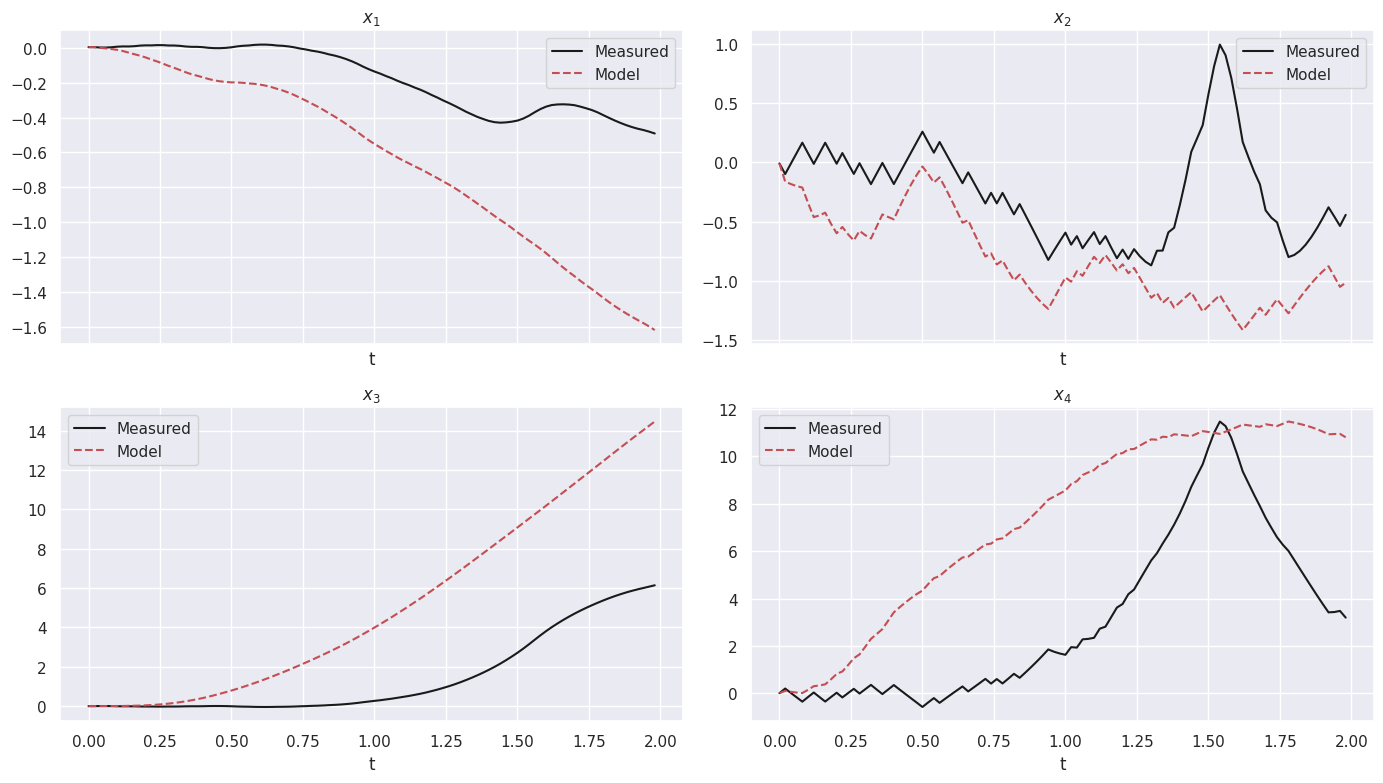
Inverted Pendulum

Exercise

Exercise 7 (Inverted Pendulum)

Use the SINDYc and/or DMDc method to fit a model on the data collected from the inverted pendulum environment.

Solution to ( 7

Show code cell content Hide code cell content

inverted_pendulum_env = create_inverted_pendulum_environment(
    max_steps=100, theta_threshold=np.inf
)

inverted_pendulum_observations = dict()
inverted_pendulum_actions = dict()
controllers = dict()

for i in range(5):
    controllers[f"PRBS {i}"] = PRBSController(
        np.asarray([(-1) ** i * inverted_pendulum_env.force_max / (2**i)]), seed=i
    )

for controller_name, controller in controllers.items():
    result = simulate_environment(inverted_pendulum_env, controller=controller)
    inverted_pendulum_observations[controller_name] = result.observations
    inverted_pendulum_actions[controller_name] = result.actions

error: XDG_RUNTIME_DIR not set in the environment.

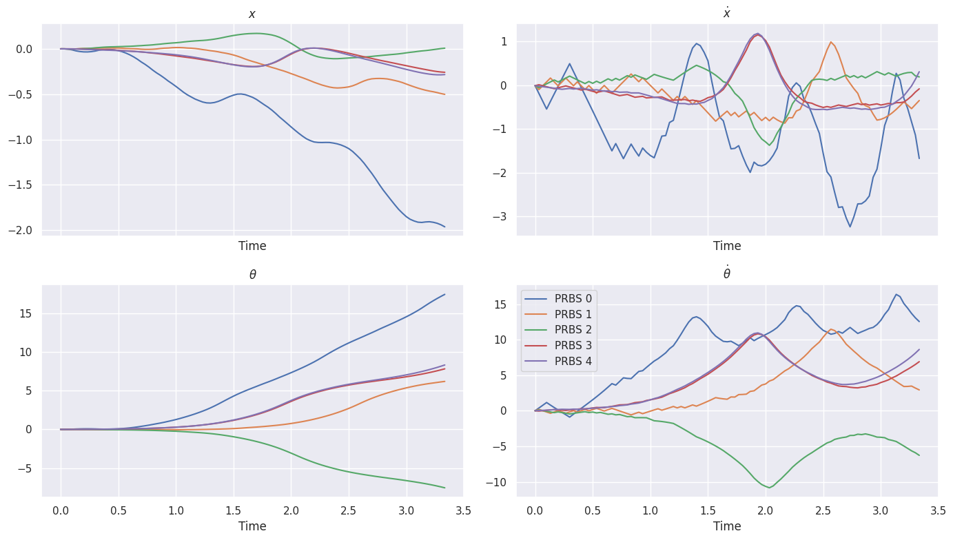
training_controller_name = "PRBS 0"
testing_controller_name = "PRBS 1"

X_train = inverted_pendulum_observations[training_controller_name][:-1].copy()
U_train = inverted_pendulum_actions[training_controller_name].copy()
t_train = np.arange(0, len(X_train)) * inverted_pendulum_env.dt

X_val = inverted_pendulum_observations[testing_controller_name][:-1].copy()
U_val = inverted_pendulum_actions[testing_controller_name].copy()
t_val = np.arange(0, len(X_val)) * inverted_pendulum_env.dt

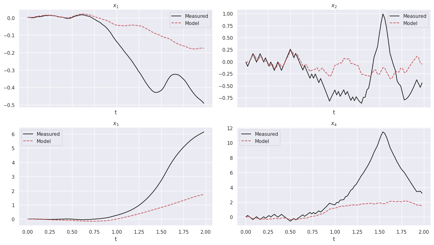
SINDYc

Show code cell source Hide code cell source

optimizer = ps.STLSQ(threshold=0.3, max_iter=500)

feature_library = ps.IdentityLibrary()

differentiation_method = ps.FiniteDifference(order=1)
sindy_model = ps.SINDy(
    optimizer=optimizer,
    feature_library=feature_library,
    differentiation_method=differentiation_method,
)
sindy_model.fit(X_train, u=U_train, t=inverted_pendulum_env.dt)

SINDy(differentiation_method=FiniteDifference(order=1),
      feature_library=<pysindy.feature_library.identity_library.IdentityLibrary object at 0x7ff73efa0a30>,
      feature_names=['x0', 'x1', 'x2', 'x3', 'u0'],
      optimizer=STLSQ(max_iter=500, threshold=0.3))

In a Jupyter environment, please rerun this cell to show the HTML representation or trust the notebook.
On GitHub, the HTML representation is unable to render, please try loading this page with nbviewer.org.

(x0)' = 0.998 x1
(x1)' = -51.462 x0 + -1.826 x1 + -5.233 x2 + -0.885 x3 + 0.651 u0
(x2)' = 1.001 x3
(x3)' = -107.086 x0 + -5.116 x1 + -12.393 x2 + -0.517 x3 + -0.698 u0

Model score: 32.144658

X_sindy = sindy_model.simulate(X_val[0], t_val, u=U_val)
X_sindy = np.vstack([X_val[0][np.newaxis, :], X_sindy])

DMDc

Show code cell source Hide code cell source

regressor = pk.regression.EDMDc()
observables = pk.observables.Polynomial(degree=1)
dmd_model = pk.Koopman(observables=observables, regressor=regressor)
dmd_model.fit(X_train, u=U_train, dt=inverted_pendulum_env.dt)

/opt/conda/lib/python3.10/site-packages/sklearn/utils/deprecation.py:103: FutureWarning: The attribute `n_input_features_` was deprecated in version 1.0 and will be removed in 1.2.
  warnings.warn(msg, category=FutureWarning)
/opt/conda/lib/python3.10/site-packages/sklearn/utils/deprecation.py:103: FutureWarning: The attribute `n_input_features_` was deprecated in version 1.0 and will be removed in 1.2.
  warnings.warn(msg, category=FutureWarning)
/opt/conda/lib/python3.10/site-packages/sklearn/utils/deprecation.py:103: FutureWarning: The attribute `n_input_features_` was deprecated in version 1.0 and will be removed in 1.2.
  warnings.warn(msg, category=FutureWarning)
/opt/conda/lib/python3.10/site-packages/sklearn/utils/deprecation.py:103: FutureWarning: The attribute `n_input_features_` was deprecated in version 1.0 and will be removed in 1.2.
  warnings.warn(msg, category=FutureWarning)

Koopman(observables=Polynomial(degree=1), regressor=EDMDc())

In a Jupyter environment, please rerun this cell to show the HTML representation or trust the notebook.
On GitHub, the HTML representation is unable to render, please try loading this page with nbviewer.org.

\[\begin{split}\displaystyle \begin{equation*}A = \begin{bmatrix}0.999999999999963 &-1.6207781644572705e-13 &-6.5658741464635906e-15 &-2.0557015291411407e-14 &2.6151024162986147e-15 \\-1.165458063723047e-09 &0.9999999964558379 &0.020000001184556554 &-6.244138547104919e-10 &3.7563398753760245e-10 \\-0.08739214280376793 &-1.0721709694682215 &0.9476892092479134 &-0.11251502064813125 &-0.00922556696486635 \\5.0851957901859835e-09 &-1.019768218902813e-08 &-3.243666745672972e-10 &0.9999999990662863 &0.019999999431521833 \\0.027640755572805417 &-2.1680865930988924 &-0.08973096067741987 &-0.2439059002560893 &0.9839030164862272 \\\end{bmatrix}\end{equation*}\end{split}\]

\[\begin{split}\displaystyle \begin{equation*}B = \begin{bmatrix}-5.082739784612045e-16 \\-9.7208605406143e-11 \\0.012240554215487356 \\1.654690707668953e-09 \\-0.014546219966763462 \\\end{bmatrix}\end{equation*}\end{split}\]

\[\begin{split}\displaystyle \begin{equation*}C = \begin{bmatrix}0.0 &1.0 &0.0 &0.0 &0.0 \\0.0 &0.0 &1.0 &0.0 &0.0 \\0.0 &0.0 &0.0 &1.0 &0.0 \\0.0 &0.0 &0.0 &0.0 &1.0 \\\end{bmatrix}\end{equation*}\end{split}\]

\[\begin{split}\displaystyle \begin{equation*}W = \begin{bmatrix}(-0.007950742882235143-0.0539261529692824j) &(-0.007950742882235143+0.0539261529692824j) &(-0.08185125670261548-0.0021262378238662964j) &(-0.08185125670261548+0.0021262378238662964j) &(-0.11043983363884793+0j) \\(0.43942433872018216+0.030507373741592934j) &(0.43942433872018216-0.030507373741592934j) &(0.00015945250410232402-0.06714666035158207j) &(0.00015945250410232402+0.06714666035158207j) &(1.5988447853804014e-08+0j) \\(-0.023554399050895656-0.10750223627039948j) &(-0.023554399050895656+0.10750223627039948j) &(0.7688918882785541+0j) &(0.7688918882785541+0j) &(0.9907039819515358+0j) \\(0.8893215199709776+0j) &(0.8893215199709776+0j) &(0.01487734526015245+0.6303737623068534j) &(0.01487734526015245-0.6303737623068534j) &(-3.025819262328861e-08+0j) \\\end{bmatrix}\end{equation*}\end{split}\]

X_dmd = dmd_model.simulate(X_val[0], U_val, n_steps=X_val.shape[0] - 1)
X_dmd = np.vstack([X_val[0][np.newaxis, :], X_dmd])

/opt/conda/lib/python3.10/site-packages/sklearn/utils/deprecation.py:103: FutureWarning: The attribute `n_input_features_` was deprecated in version 1.0 and will be removed in 1.2.
  warnings.warn(msg, category=FutureWarning)
/opt/conda/lib/python3.10/site-packages/pykoopman/koopman.py:302: ComplexWarning: Casting complex values to real discards the imaginary part
  x = x.astype(self.A.dtype)

Model score: 11.334027

---

[1]

The step response of a dynamic system is its output when presented with an input signal, called step, that changes from 0 to a constant values in a very short amount of time.

[2]

The impulse response of a dynamic system is its output when presented with a brief input signal, called an impulse. Any LTI system can be uniquely characterized by its impulse response

[3]

A phase portrait is a geometric representation of the trajectories of a dynamical system in the phase plane. Each set of initial conditions is represented by a different curve, or point.

[4]

The Frobenius norm of a matrix \(\mathbf{X} \in \mathbb{C}^{m\times n}\) is defined as \(\left\lVert \mathbf{X} \right\rVert_F = \sqrt{\sum_{i=0}^{m} \sum_{j=0}^{n} x_{i,j}}\)

[5]

\(R^2\) values range from 0 to 1. An R-Squared value of 0 means that the model explains or predicts 0% of the relationship between the dependent and independent variables. A value of 1 indicates that the model predicts 100% of the relationship.